What is Image Processing? - Great Learning

Introduction to Image Processing
Libraries involved for an Image Processing
Why do we need Image Processing?
Steps in Image Processing
Pre-requisites
Installation of Libraries
Image Processing with OpenCV
Applications in Image Processing – A Case Study

Introduction to Image Processing

Image processing is a way to convert an image to a digital aspect and perform certain functions on it, in order to get an enhanced image or extract other useful information from it. It is a type of signal time when the input is an image, such as a video frame or image and output can be an image or features associated with that image. Usually, the AWS Image Processing system includes treating images as two equal symbols while using the set methods used.

It is one of the fastest growing technologies today, with its use in various business sectors. Graphic Design forms the core of the research space within the engineering and computer science industry as well.

Image processing basically involves the following three steps.

Importing an image with an optical scanner or digital photography.

Analysis and image management including data compression and image enhancement and visual detection patterns such as satellite imagery.

It produces the final stage where the result can be changed to an image or report based on image analysis.

Image processing is a way by which an individual can enhance the quality of an image or gather alerting insights from an image and feed it to an algorithm to predict the later things.

Libraries involved in Image Processing

The following libraries are involved in performing Image processing in python;

Scikit-image
OpenCV
Mahotas
SimplelTK
SciPy
Pillow
Matplotlib

scikit-image is an open-source Python package run by the same NumPy members. It uses algorithms and resources for research, academic and industrial use. It is a simple and straightforward library, even for newcomers to Python’s ecosystem. The code is high quality, reviewed by peers, and written by a working community of volunteers.

Scikit Image Documentation: https://scikit-image.org/docs/stable/

SciPy is one of Python’s basic science modules (like NumPy) and can be used for basic deception and processing tasks. In particular, the submodule scipy.ndimage (in SciPy v1.1.0) provides functions that work on n-dimensional NumPy arrays. The package currently includes direct and offline filtering functions, binary morphology, B-spline translation, and object ratings.

SciPy Documentation: https://www.scipy.org/docs.html

PIL (Python Imaging Library) is a free Python programming language library that adds support for opening, managing, and storing multiple image file formats. However, its development has stalled, with the last release in 2009. Fortunately, there is a Pillow, a PIL-shaped fork, easy to install, works on all major operating systems, and supports Python 3. Color-space conversions.

Pillow Documentation: https://pillow.readthedocs.io/en/3.1.x/index.html

Enhancing an image in Pillow using ImageFilter

OpenCV (Open Source Computer Vision Library) is one of the most widely used libraries in computer programming. OpenCV-Python is an OpenCV Python API. OpenCV-Python is not only running, because the background has a code written in C / C ++, but it is also easy to extract and distribute (due to Python folding in the front). This makes it a good decision to make computer vision programs more robust.

OpenCV Documentation: https://docs.opencv.org/master/d6/d00/tutorial_py_root.html

Image blending using Pyramids in OpenCV-Python

Mahotas is another Python computer and graphics editor. It contains traditional image processing functions such as morphological filtering and functioning, as well as modern computer-assisted computational computation functions, including the discovery of point of interest and local definitions. The display is in Python, which is suitable for rapid development, but the algorithms are used in C ++ and are fixed at speed. The Mahotas Library is fast with little code and with little reliance.

Mahotas Documentation: https://mahotas.readthedocs.io/

ITK (Insight Segmentation and Registration Toolkit) is an open-source, shortcut system that provides developers with a comprehensive set of image analysis software tools. and translated languages. “It is also an image analysis tool with a large number of features that support the functionality of standard filtering, image classification, and registration. SimpleITK is written in C ++ but is available in a large number of programming languages including Python.

SimpleITK Documentation: https://simpleitk.readthedocs.io/en/master/

Why do we need Image Processing?

Image processing is often regarded as improperly exploiting the image in order to achieve a level of beauty or to support a popular reality. However, image processing is most accurately described as a means of translation between a human viewing system and digital imaging devices. The human viewing system does not see the world in the same way as digital cameras, which have additional sound effects and bandwidth. Significant differences between human and digital detectors will be demonstrated, as well as specific processing steps to achieve translation. Image editing should be approached in a scientific way so that others can reproduce, and validate human results. This includes recording and reporting processing actions and applying the same treatment to adequate control images.

Steps in Image Processing

Image Acquisition: This is the first digital step in image processing. Digital image detection to create specific images, such as a real or real situation internal arrangement of an object. This word is commonly expected to accept processing, congestion, storage, printing, and display of such images. Image acquisition may humble as considering the pre-existing image digital form.

Image Enhancement: Image enhancement is a process of switching digital images to more results suitable for display or multiple image analysis. Because for example, you can turn off sound, sharpen, or turn on image, which makes it easier to identify key features.

Image Restoration: Image Restoration is a function of taking anunethical / noisy image and measuring an unused, new image. Exploitation can occur in many ways such as action blurring, sound and camera focus The purpose of image restoration techniques is to reduce noise and reclaim the loss of decision.

Coloring Image Processing: Color Image Processing it requires an understanding of the physics of light as well color vision phycology. The color of human use details of classification of materials, building materials, food, places and time of day. Color for the purpose of separation image processing process is used.

Wavelets Processing and Multiple Solutions: When Decorated photo thru atmosphere, clouds, trees, and flowers, you will use a different level brush depending on the size of topographies. Wavelets are likened to those brushes. Wavelets transform is an effective tool for image representation. The wavelet transform allows for the investigation of multiple solutions of the image.

Image compression: Image compression is a type of data useful pressure digital photography, reducing their costs last or spread. Processes can reap visual benefits awareness and asset data image assets to complex effects related to normal pressure strategies.

Character recognition: Optical character binding, commonly accessed by OCR, machine operated or electronic replacement of scanned images or kindly or typed text that is, computer-readable text. It is often used as a presence to access records from the minute a new type of data source, whether paper, invoice, bank statement, income, business cards, number of printed records or email. It’s a common way to make digital printed manuscripts such as those that can be by electronic means sorted, searched, and stored in the machine processes such as machine conversion and display online, text-to-speech, retrieval of key data and text mining. OCR is a plethora of research on intelligence, pattern and computer concept.

Pre-requisites

Before we move on, let’s talk about what you need to know in order to follow this lesson easily. First, you should have a basic knowledge of the program in any language. Second, you need to know what reading materials are and what the basics are for how they work, as we will be using other machine learning algorithms for this image processing. As a bonus, it may help if you have experienced exposure, or basic Open CV information before continuing with this course. But this is not necessary.

One thing you should definitely know following this tutorial is how the image is represented in memory. Each image is represented by a set of pixels i.e. a matrix of pixel values. In the gray image, the pixel values range from 0 to 255 and represent the intensity of that pixel. For example, if you had a 20 x 20 size image, it would be represented by a 20×20 matrix (total value of 400 pixels).

If you are working with a color image, you should know that we will have three channels – Red, Green, and Blue (RGB). Therefore, there will be three such matrices for one image.

This post is a humble effort to get people interested in this place and by using a simple example, show how easy it is to get started. All we need is a working Python knowledge and a small OpenCV domain.

Python – Although there are many courses available online, personally, I found dataquest .io to be a great python learning platform, for beginners and experienced alike.

OpenCV – Similar to python, OpenCV also has many online tutorials. The only site I find that I often talk about is the official documents.

HaaR Cascades – OpenCV unveils special ways to train our custom algorithms to find anything interesting in image capture. HaaR cascade are those files that contain that trained model.

Installation of Libraries

To run any of the above packages mentioned in “Libraries involved in Image Processing” please make sure you have the recent version of Python 3.x installed on your local machine. However, the code in this blog can be also run on Google Colab or any other cloud service having Python Interpreter.

For Windows system;

pip install opencv-python

pip install scikit-image

pip install mahotas

pip install scipy

pip install Pillow

pip install matplotlib

For Linux;

sudo apt-get install libopencv-dev python-opencv

sudo apt-get install python-skimage

sudo apt-get install python-mahotas

sudo apt-get install python-scipy

sudo apt-get install python-Pillow

sudo apt-get install python-matplotlib

For MacOS;

brew install opencv3 –with-contrib –with-python3 :

https://stackoverflow.com/questions/1213690/what-is-the-most-compatible-way-to-install-python-modules-on-a-mac

To cross-check whether or not the packages were installed in your machine, you can type the following;

import package_name

If this doesn’t give out an error saying the header file is not present then you’re good to go!

Data Science Toolkit

https://www.anaconda.com/products/individual

Image Processing with OpenCV

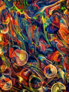
Actual Image

#Import the Header File

import cv2

#Reading Image file from File Location

img = cv2.imread(‘image.jpg’)

#Functions to find out generic properties of an Image

print("Image Properties") 
print("Number of Pixels: " + str(img.size)) 
print("Shape/Dimensions: " + str(img.shape))

#Output

Image Properties

Number of Pixels: 60466176

Shape/Dimensions: (5184, 3888, 3)

import cv2
import numpy as np
from matplotlib import pyplot as plt
img = cv2.imread('image.jpg') // Combination of all colors 
b,g,r = cv2.split(img)       # get b,g,r
rgb_img = cv2.merge([r,g,b])
plt.imshow(rgb_img)
x,y,z = np.shape(img)
red = np.zeros((x,y,z),dtype=int)
green = np.zeros((x,y,z),dtype=int)
blue = np.zeros((x,y,z),dtype=int)
for i in range(0,x):
    for j in range(0,y):
        red[i][j][0] = rgb_img[i][j][0]
        green[i][j][1]= rgb_img[i][j][1]
        blue[i][j][2] = rgb_img[i][j][2]
 
 
plt.imshow(red)  // red color image ( fig 2)
plt.imshow(green)  // green color image ( fig 3)
plt.imshow(blue)  // Blue color image ( fig 4)
#Now we will again create the original image from these Red, Blue and Green Images
retrack_original = np.zeros((x,y,z),dtype=int)
for i in range(0,x):
    for j in range(0,y):
        retrack_original[i][j][0] = red[i][j][0]
        retrack_original[i][j][1] = green[i][j][1]
        retrack_original[i][j][2] = blue[i][j][2]
cv2.imwrite('ori.jpg',retrack_original) 
plt.imshow(retrack_original)

From the above code

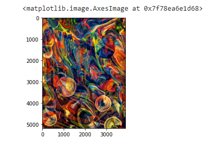
Fig 1: Combination of all colors

Fig 2: Red color

Fig 3 : Green Color

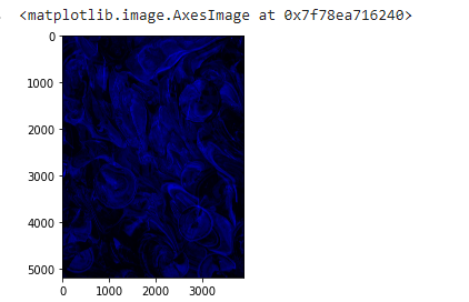
Fig 4: Blue Color

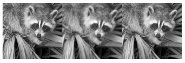
How to Convert an Image into its equivalent grayscale version?

import cv2 as cv
import numpy as np
import matplotlib.pyplot as plt
 
img = cv.imread('image.jpg')
gray_image = cv.cvtColor(img, cv.COLOR_BGR2GRAY)
 
fig, ax = plt.subplots(1, 2, figsize=(16, 8))
fig.tight_layout()
 
ax[0].imshow(cv.cvtColor(img, cv.COLOR_BGR2RGB))
ax[0].set_title("Original")
 
ax[1].imshow(cv.cvtColor(gray_image, cv.COLOR_BGR2RGB))
ax[1].set_title("Grayscale")
plt.show()

Separating each Color Channel in an Image

b, g, r = cv.split(img)
 
fig, ax = plt.subplots(1, 3, figsize=(16, 8))
fig.tight_layout()
 
ax[0].imshow(cv.cvtColor(r, cv.COLOR_BGR2RGB))
ax[0].set_title("Red")
 
ax[1].imshow(cv.cvtColor(g, cv.COLOR_BGR2RGB))
ax[1].set_title("Green")
 
ax[2].imshow(cv.cvtColor(b, cv.COLOR_BGR2RGB))
ax[2].set_title("Blue")

Image Translation

h, w = img.shape[:2]
 
half_height, half_width = h//4, w//8
transition_matrix = np.float32([[1, 0, half_width],
                               [0, 1, half_height]])
 
img_transition = cv.warpAffine(img, transition_matrix, (w, h))
 
plt.imshow(cv.cvtColor(img_transition, cv.COLOR_BGR2RGB))
plt.title("Translation")
plt.show()

Image Rotation

h, w = img.shape[:2]
 
rotation_matrix = cv.getRotationMatrix2D((w/2,h/2), -180, 0.5)
 
rotated_image = cv.warpAffine(img, rotation_matrix, (w, h))
 
plt.imshow(cv.cvtColor(rotated_image, cv.COLOR_BGR2RGB))
plt.title("Rotation")
plt.show()

Scaling and Resizing of Image

fig, ax = plt.subplots(1, 3, figsize=(16, 8))
 
# image size being 0.15 times of it's original size
image_scaled = cv.resize(img, None, fx=0.15, fy=0.15)
ax[0].imshow(cv.cvtColor(image_scaled, cv.COLOR_BGR2RGB))
ax[0].set_title("Linear Interpolation Scale")
 
# image size being 2 times of it's original size
image_scaled_2 = cv.resize(img, None, fx=2, fy=2, interpolation=cv.INTER_CUBIC)
ax[1].imshow(cv.cvtColor(image_scaled_2, cv.COLOR_BGR2RGB))
ax[1].set_title("Cubic Interpolation Scale")
 
# image size being 0.15 times of it's original size
image_scaled_3 = cv.resize(img, (200, 400), interpolation=cv.INTER_AREA)
ax[2].imshow(cv.cvtColor(image_scaled_3, cv.COLOR_BGR2RGB))
ax[2].set_title("Skewed Interpolation Scale")

Blurring an image using Pillow

from PIL import Image
from PIL import ImageFilter
# Open Existing Image
OrgImage = Image.open("image.jpg")
# Apply Simple Blur Filter
blurImage = OrgImage.filter(ImageFilter.BLUR)
blurImage.show()
# blurImage.save("output1.jpg")
# Apply BoxBlur Filter
boxImage = OrgImage.filter(ImageFilter.BoxBlur(2))
boxImage.show()
# boxImage.save("output2.jpg")
# Apply GaussianBlur Filter
gaussImage = OrgImage.filter(ImageFilter.GaussianBlur(2))
gaussImage.show()
# gaussImage.save("output3.jpg")

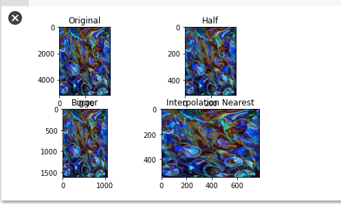
Image Rescaling

import cv2 
import numpy as np 
import matplotlib.pyplot as plt  
# This is a magic command to display in an external window 
  
image = cv2.imread("image.jpg", 1) 
# Loading the image 
  
half = cv2.resize(image, (0, 0), fx = 0.1, fy = 0.1) 
bigger = cv2.resize(image, (1050, 1610)) 
  
stretch_near = cv2.resize(image, (780, 540),  
               interpolation = cv2.INTER_NEAREST) 
  
  
Titles =["Original", "Half", "Bigger", "Interpolation Nearest"] 
images =[image, half, bigger, stretch_near] 
count = 4
  
for i in range(count): 
    plt.subplot(2, 2, i + 1) 
    plt.title(Titles[i]) 
    plt.imshow(images[i]) 
  
plt.show()

Edge Detection using Canny

import cv2
import numpy as np
from matplotlib import pyplot as plt
 
img = cv2.imread('image.jpg',0)
edges = cv2.Canny(img,100,200)
 
plt.subplot(121),plt.imshow(img,cmap = 'gray')
plt.title('Original Image'), plt.xticks([]), plt.yticks([])
plt.subplot(122),plt.imshow(edges,cmap = 'gray')
plt.title('Edge Image'), plt.xticks([]), plt.yticks([])
 
plt.show()

Enhancing Image using PIL – Pillow

from PIL import Image,ImageFilter  
#Read image
im = Image.open('image.jpg')
#Display image  
im.show()
from PIL import ImageEnhance  
enh = ImageEnhance.Contrast(im)  
enh.enhance(1.8).show("30% more contrast")

Applications of Image Processing

1. Intelligent Transportation Systems – This method can be used for automatic number identification and identification of Traffic signs.

2. Remote Sensing – In this application, the sensors take pictures of the earth’s surface on remote sensing satellites or a multi-screen scanner mounted on an aircraft. These images are processed by transfer to a global channel. Strategies used to translate materials and regions are used for flood management, town planning, resource mobilization, monitoring agricultural production, etc.

3. Moving a tracking object – This app enables you to measure movement limits and get a visual record of a moving object. The different types of tracking are:

· Active tracking

· Awareness based on awareness

4. Security monitoring – Aerial surveillance systems are used to monitor land and sea. This application is used to determine the types and configurations of submarines. An important function is to distinguish the various elements present in the body of the water body of the image. Different parameters such as length, width, area, perimeter, cohesion are set to separate each separated item. It is important to note the distribution of these items on the various sides east, west, north, south, north-east, northwest, south-east and southwest in order to define the entire shipping structure. We can interpret the whole oceanic situation from the local distribution of these things.

5. Automatic Testing Program – This application improves the quality and productivity of the product in the industry.

Automatic testing of incandescent lamp fibers – This includes testing of the process of making a lamp. Because of the variability in the height of the cord in the lamp, the lump cord is connected during a short time. In this application, a piece of binary image of a string is created on which the silhouette of a filament is formed. Silhouettes are analyzed to determine the difference in height of the lamp in the lamp. The system is operated by General Electric Corporation.

· Automatic face testing systems – In the metal industry it is important to detect local faults. For example, it is important to detect any deviation from the metal object wrapped in hot or cold grinding plants on metal plants. Image processing techniques such as texture detection, edge detection, fractal analysis etc. are used for detection.

Wrong Identification – This application identifies incorrect items in electrical or electronic systems. A high amount of heat energy is caused by these faulty components. Infra red images are produced by the distribution of heat energy in the assembly. Errors can be detected by analyzing infrared red images.

Colour Detection using OpenCV-Python

Steps to complete the project along with source code;

Step 1: Install the required libraries i.e.e CV2, Numpy, Pandas, and aargparse by referring to the library installation section covered in the above sections.

import cv2

import numpy as np

import pandas as pd

import argparse

Step 2: In this python program we will be using run time arguments to take image file dynamically from the user input from the Command prompt.

Step 3: Start reading the CSV file. (colors.csv).

csv = pd.read_csv(‘colors.csv’, names=index, header=None)

Step 4: Understanding what’s there in the CSV file. Perform .info() method on the data to look out for the datatypes and values present.

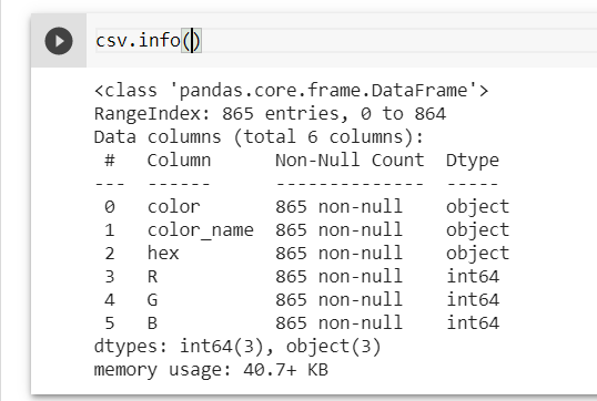
Step 5: To check for null value treatment we have to use isna() along with sum() function to find out the number of null values present in the csv file.

Step 6: Understanding the Code.

Here, the variable “ap” consists of argparse which helps us take the dynamic image input using -i <image_name> which gives the user chance to give any image of his choice.

#Creating argument parser to take image path from command line

ap = argparse.ArgumentParser()

ap.add_argument(‘-i’, ‘–image’, required=True, help=”Image Path”)

args = vars(ap.parse_args())

img_path = args[‘image’]

The variable “Clicked” here refers to the cursor movement and clicks over the image for the python code to process the image and tell which color is it.

By default, the position for Red, Green and Blue is 0

To check the type of data present in the csv file, we can check the first five records in python using .head().

The “index” variables have parameters/attributes defined in the sequence of the data headers in CSV.

#Reading the image with opencav
img = cv2.imread(img_path)
 
#declaring global variables (are used later on)
clicked = False
r = g = b = xpos = ypos = 0
 
 
#Reading csv file with pandas and giving names to each column
index=["color","color_name","hex","R","G","B"]
 
#function to calculate minimum distance from all colors and get the most matching color
def getColorName(R,G,B):
    minimum = 10000
    for i in range(len(csv)):
        d = abs(R- int(csv.loc[i,"R"])) + abs(G- int(csv.loc[i,"G"]))+ abs(B- int(csv.loc[i,"B"]))
        if(d<=minimum):
            minimum = d
            cname = csv.loc[i,"color_name"]
    return cname
 
#function to get x,y coordinates of mouse double click
def draw_function(event, x,y,flags,param):
    if event == cv2.EVENT_LBUTTONDBLCLK:
        global b,g,r,xpos,ypos, clicked
        clicked = True
        xpos = x
        ypos = y
        b,g,r = img[y,x]
        b = int(b)
        g = int(g)
        r = int(r)
       
cv2.namedWindow('image')
cv2.setMouseCallback('image',draw_function)
 
while(1):
 
    cv2.imshow("image",img)
    if (clicked):
   
        #cv2.rectangle(image, startpoint, endpoint, color, thickness)-1 fills entire rectangle 
        cv2.rectangle(img,(20,20), (750,60), (b,g,r), -1)
 
        #Creating text string to display( Color name and RGB values )
        text = getColorName(r,g,b) + ' R='+ str(r) +  ' G='+ str(g) +  ' B='+ str(b)
        
        #cv2.putText(img,text,start,font(0-7),fontScale,color,thickness,lineType )
        cv2.putText(img, text,(50,50),2,0.8,(255,255,255),2,cv2.LINE_AA)
 
        #For very light colours we will display text in black colour
        if(r+g+b>=600):
            cv2.putText(img, text,(50,50),2,0.8,(0,0,0),2,cv2.LINE_AA)
            
        clicked=False
 
    #Break the loop when user hits 'esc' key    
    if cv2.waitKey(20) & 0xFF ==27:
        break
    
cv2.destroyAllWindows()

Function getColorName(R,G,B)

This function runs for the entire number of records in the csv file and stores the absolute values of differences between the given Red, Green and Blue in the image Vs the actual R,G,B color spectrum. If the absolute value is less than the bare minimum value then the color name will have the equivalent name from location of that color as given in the csv.

We have the values of r, g and b. Now, we need another function that will restore the color name from RGB values. To find the color name, we calculate the distance (d) that tells us how close we are to coloring and select the one with the lowest distance.

Function draw_function()

It will calculate the double-click rgb pixel values. Activity parameters with event name, (x, y) mouse status links, etc. In the function, we check whether the event is double-clicked and calculate and set the values r, g, b and x, y the position of the mouse.

Whenever a two-click event occurs, it will update the color name and RGB values in the window.

Using the cv2.imshow () function, we draw a picture in a window. When a user double-clicks a window, we draw a rectangle and find the color name to draw the text in the window using the cv2.rectangle and cv2.putText () functions.

In this Python project with source code, we learned about colours and how to extract RGB colour values and pixel colour name. We learned to manage events such as double-clicking in a window and saw how to read CSV files with pandas and perform tasks on data. This is used for many photo editing and drawing applications.

Applications in Image Processing

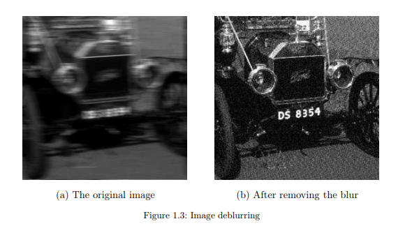
Image Processing with MATLAB

What is MATLAB?

MATLAB is used as part of laboratory exercises and problem categories in photography

Processes half of the unit unit for Computer Graphics and Image Processing. This brochure explains the MATLAB development environment you will use, you are expected to learn and become familiarize yourself with it before attempting Laboratory Assignments and Study Activities. MATLAB is a data analysis and visualization tool designed to make matrix fraud as easy asit is possible. In addition, it has strong graphics capabilities and its own programming language. The basic MATLAB distribution can be expanded by adding a list of toolboxes, corresponding to Of course an image processing toolbox (IPT). Basic distribution and everything currently available toolboxes are available in labs. Basic distribution and any toolboxes included will provide a large selection of functions, requested through the command line interface.

The basic data structure of MATLAB is matrix1. In MATLAB one flexibility is 1 x 1 matrix, thread is 1 x n matrix of charts. The image is an n x m matrix of pixels.

MATLAB’s development Environment

IMLL is started within the Windows environment by clicking on the icon that should be in it

desktop. (MATLAB is available for Linux and MacOS, but these sites are not supported

in laboratories, and these versions have their own license arrangements that can be integrated

University license.)

MATLAB IDE has five components: Command Window, Workspace Browser, Current

Guide Window, Windows Command History Window and zero or more active Figure Windows

display only graphical objects.

The Command window is where commands and commands are typed, and the results are presented as appropriate.

Workspace is a set of variables created during a session. They are shown in the file

Workspace Browser. More details on the variety are available there, some variables may also apply editing.

The current cursor window shows the contents of the current active directory and methods

past performance indicators. The active directory can be changed. MATLAB uses the search method to find files. The search method includes the current directory, all toolboxes included and more user add-ons – using the Set Path dialog that is accessible from the file menu.

The command history window provides an overview of current and past session history. Instructions appearing here can be redone.

Image Representation in MATLAB

Image Format

Image Loading and Displaying and Saving

>> f = imread(‘image file name’);

Grey Level Ranges

mages are usually captured in pixels on each channel represented by eight integers. (This

in part due to historical reasons – it has the potential to be a basic memory unit, allowing a

the appropriate price range will be represented, and many cameras could not enter data into any large one accuracy. In addition, multiple displays are limited to eight bits per red, green and blue channel.)

There is no reason why pixels should be limited, of course, there are devices and applications that also deliver requires high resolution data. MATLAB supports the following types of data.

Type/ Interpretation/ Range

uint8/ unsigned 8-bit integer / [0, 255]

uint16/ unsigned 16-bit integer/ [0, 65535]

uint32/ unsigned 32-bit integer / [0, 4294967295]

int8/ signed 8-bit integer / [-128, 127]

int16/ signed 16-bit integer/ [-32768, 32767]

int32/ signed 32-bit integer / [-2147483648, 2147483647]

single/ single precision floating point number / [-1038, 1038]

double/ double precision floating point number/ [-10308, 10308]

char/ character / (2 bytes per element)

logical values/ are /0 or 1 1 byte per element

An image is often translated as one of: solid, binary, indexed or RGB. Solid image values reflect light. Binary image pixels have only two possibilities prices. The displayed pixel values are treated as an “true” reference table. number read. RGB images have three channels, representing the maximum range of wavelengths accompanied by red, green and blue lighting (some wavelengths and more possible).

MATLAB provides functions for changing images from one type to another. The syntax is

>> B = data_class_name(A)

where data_class_name is one of the data types in the above table, e.g.

>> B = uint8(A)

will convert image A (of some type) into image B of unsigned 8-bit integers, with possible loss of

resolution (values less than zero are fixed at zero, values greater than 255 are truncated to 255.)

Functions are provided for converting between image types, in which case the data is scaled to fit the

new data type’s range. These are defined to be:

Function/ Input Type/ Output Type/

im2uint8 Logical/ uint8, uint16/ double Unint8/

im2uint16 Logical/ uint8, uint16/ double Uint16/

mat2gray double Double in range [0, 1]

im2double Logical/ uint8, uint16/ double Double/

im2bw/ Uint8 uint16, double logical/

Basics of MATLAB

To read an image in MATLAB we can start by using imread() method in the MATLAB console.

>> variable_name = imread(“picture_name.extension”);
>> w=imread(’wombats.tif’);

To get a size of a image in MATLAB you can write the command,

>> [M,N]=size(f)

The imshow() function, It should be noted that in a ‘double’ type matrix, the imshow function expects values to be between 0 and 1, where 0 is shown as black and 1 as white. Any value between 0 and 1 is shown as a dimension. Any number greater than 1 is shown as white, and a value less than zero is shown as black. To find values within this range, a separator can be used. The larger the distinguishing feature, the darker the image.

For example, if you give the command impression (G), the image displayed on the desktop is provided in Fig. 3. ‘imshow (F)’ shows the image shown in Fig. 4. ‘imshow (f, [high, low)’ which shows in black all the values that are lower or equal to ‘low’ and white which are all values equal to or greater than ‘high.’ Medium values are expressed as intermediate strength values.

‘Imshow (f, [])’ sets the variable down to the minimum number of the same members ‘f’ and rises to its maximum value. This helps to improve the contrast of low-density images.

The image tool in the image processing toolbox provides a highly interactive environment for viewing and navigating within images, showing detailed information on pixel values, measurement distances and other useful functions. To start the image tool, use the imtool function. The following statements read the Penguins_grey.jpg image saved to the desktop and showed it to us using ‘imtool’:

>>B = imread(Penguins_grey.jpg);
>>imtool(B)

Multiple images can be displayed within a single number using the function below. This function has three parameters within brackets, where the first two parameters specify the number of rows and columns for dividing a number. The third parameter specifies which classification should be used. For example, a subplot (3,2,3) tells MATLAB to divide a number into three rows with two columns and set the third cell as active. To display images Penguins_RGB.jpg and Penguins_grey.jpg merge into one image, you need to provide the following instructions:

>> A=imread(‘Penguins_grey.jpg’);
>> B=imread(‘Penguins_RGB.jpg’);
>>figure
>>subplot(1,2,1),imshow(A)
>>subplot(1,2,2),imshow(B)

Writing Images

>> imwrite(f,’filename’)

>> imwrite(f,’filename.jpg’, ‘quality’,q)

Here the quality variable i.e. “q” lies somewhere between 0 and 100, it can be implied on decreasing the image size, however, it’s a trade-off between quality and file size.

>> F = imread(‘Penguins_grey.jpg’);
>> imwrite(F,’Penguins_grey_75. jpg’,’quality’,75);
>> imwrite(F,’Penguins_grey_10. jpg’,’quality’,10);
>> imwrite(F,’Penguins_grey_90. jpg’,’quality’,90);

The file details MATLAB can be extracted by using the following function;

>>imfinfo ’filename’

>> K = imfinfo(‘Penguins_grey.jpg’)

Image processing includes many methods and a variety of techniques and algorithms. The basic techniques that support these techniques include sharpening, noise removal, minimization, edge removal, visibility, comparison enhancement, and object classification and labeling

Sharpening enhances the edges and fine details of an image for public viewing. It enhances the contrast between light and dark regions to bring out the features of the image. Basically, sharpening involves the use of a high-resolution filter in the image.

Sound removal techniques reduce the amount of noise in the image before it is processed. Required for image processing and image translation to obtain useful information. Photos from both digital cameras and standard video cameras capture sound from a variety of sources. These sound sources include the sound of salt and pepper (low light and dark distortion) and Gaussian sound (each pixel value in an image changes in a small amount). In any case, the sound of different pixels may or may not be mixed. In most cases, sound values in different pixels are modeled as independent and evenly distributed and are therefore related. In choosing an audio reduction algorithm, one should consider the computer’s power and time available and whether the provision of certain image details is acceptable if it allows a large amount of sound to be removed and so on.

Redesigning the process of removing the blurring process (such as blurring caused by defocus aberration or motion blur) in images. Blur is modeled as a convolution point distribution function with a sharp input image, where both sharp image (to be obtained) and the point distribution function are unknown. Deblurring algorithms include a way to clear the blur in the image. Deblurring is an iterative process and you may need to repeat the process several times until the final image is a good measure of the original image.

Edge extraction or edge detection is used to separate objects from each other before identifying their contents. Includes a variety of mathematical methods aimed at identifying points in a digital image where the brightness of the image changes significantly.

Edge acquisition methods can be categorized in terms of usage and in a method based on zero. Methods based on obtaining the edges by starting to use the edge-edge measurement (usually the function from the first order) such as gradient size and then measuring the maxima orientation of the gradient size area using a computer-based layout, usually the gradient orientation. Zero crossing methods look for zero jumps in performance based on second order combined from the image to get the edge. The first edge detectors include a cannon detector on the edge, Prewitt and Sobel operators, and so on.

Other methods include the division of the second order of obtaining zero overrides, methods of phase merging (or phase merging) or phase conversion (PST). The second-order split method detects zero exit of the second-order exit in the gradient directory. The classification methods try to find areas in the image where all the sinusoids in the common domain in the section. PST transforms the image by mimicking the spread of the opposing machine with distributed 3D material (display indicator).

Binarisation refers to lowering the greyscale image to only two levels of gray, i.e., black and white. Thresholding is a popular process of converting any greyscale image into a binary image.

Comparison enhancements were made to improve the image view of the person and the image processing functions. It makes the image features more vivid in the efficient use of colors found on the display or on the output device. Fraudulent fraud involves changing the range of comparative values in the image.

Subdivision of the object label within the scene is a requirement for multidisciplinary recognition and classification systems. Process separation is the process of assigning each pixel to a source image in two or more categories. Image segregation is the process of dividing digital image into several parts (pixel sets, also known as super pixels). The goal is to simplify and / or transform image representation into something meaningful and easy to analyze. Once the relevant items have been labeled, their relevant features can be extracted and used to classify, compare, combine or identify the required items.

Types of images

The MATLAB toolbox supports four types of images, namely, gray images, binary images, indexed images and RGB images. A brief description of these types of images is provided below.

Grayscale images

Also referred to as monochrome images, these use 8 bits per pixel, whereas 0 pixel value corresponds to ‘black,’ 255 pixel value corresponds to ‘white’ and medium values showing different shades of gray. This is coded as clusters of 2D pixels, each pixel having 8 pieces.

Binary images

These images use 1 bit per pixel, where 0 usually means ‘black’ and 1 means ‘white.’ These are represented as 2D columns. Small size is a big advantage of binary images.

Featured images

These images are a matrix of whole numbers (X), where each number refers to a specific RGB price line in the second matrix (map) known as a color map.

RGB image

In the RGB image, each color pixel is represented as three times the values of its R, G and B objects. In MATLAB, the RGB color image corresponds to the 3D dimensions of size M × N × 3. Here ‘M’ and ‘N’ are the height and width of the image, respectively, and 3 is the number of color segments. For RGB images of duplicate category, the range of values is [0.0, 1.0], and for categories un8 and uint16, ranges [0, 255] and [0, 65535], respectively.

Sharpening an image

Sharpening an image is a powerful tool for emphasizing texture and drawing the viewer’s focus. It can improve the quality of the image, even more so than the advanced camera lens.

Most sharpening tools work by inserting something called a ‘sharp mask,’ which is actually working on sharpening the image. The tool works by adding a light contrast to the inner edges of the image. Note that the sharpening process may not re-create a positive image, but creates the appearance of a well-known edge.

The command used to sharpen an image in MATLAB is:

B = remove (A)

Returns an improved version of the greyscale or true-color (RGB) image input A, in which the edges of the image such as edges have been sharpened using an obscure encryption method.

B = imsharpen (A, Name, Value,….) Sharpens the image using value-name pairs to control the features of the subtleties.

Let’s see the use of the imsharpen function:

>> a = read (‘Image_sharpen.jpg’);

>> imshow (a)

Conclusion

Image processing is a way of doing certain tasks in an image, to get an improved image or to extract some useful information from it. It is a type of signal processing where the input is an image and the output can be an image or features/features associated with that image. Today, image processing is one of the fastest-growing technologies. It creates a major research space within engineering and computer science as well. Check out the image processing course and understand the details of the image processing concept.

Image processing basically involves the following three steps:

Image import with image detection tools;

Image analysis and management;

The result of which an image or report based on image analysis can be changed.

There are two types of image processing methods, namely analogue and digital image processing. Analogue image processing can be used for hard copies such as printing and photography. Image analysts use a variety of translation bases while using these viewing methods. Digital image processing techniques facilitate the use of digital images using computers. The three common categories that all types of data are required to use when using the digital process are pre-processing, development, and display of information.

Learn more about image processing with the help of Great learning’s artificial intelligence courses and build a successful career in AI and ML.

Introduction to Image Processing | What is Image Processing?