Introduction to Stochastic Gradient Descent

Stochastic: “Process involving a randomly determined sequence of observations, each of which is considered as a sample of one element from a probability distribution.”  Or, in simple terms, “Random selection.”

Contributed by: Sarveshwaran

Points discussed:

1. Optimization
2. Optimization Function
3. Loss Function
4. Derivative
5. Optimization Methods
6. Gradient Descent
7. Stochastic Gradient Descent

What is the need of Optimization?

Any algorithm has an objective of reducing the error, reduction in error is achieved by optimization techniques.

Error: Cross-Entropy Loss in Logistic Regression, Sum of Squared Loss in Linear Regression

What is Optimization function?

Optimization is a mathematical technique of either minimizing or maximizing some function f(x) by altering x. In many real-time scenarios, we will be minimizing f(x). Well, if the thought comes up, how do we maximize the f(x)? It is just possible by minimizing the -f(x). Any function f(x) that we want to either minimize or maximize we call the objective function or criterion.

What is a Loss function?

Whenever we minimize our objective function f(x) we call it a loss function. Loss function takes various names such as Cost function or error function. 

Derivative:

Let’s take an example of a function y = f(x), where both x and y are real numbers. The derivative of this function is denoted as f’(x) or as dx/dy. The derivative f’(x) gives the slope of f(x) at the point x. In other words, it directs us how a small change in the input will correspond to the change in output. The derivative is useful to minimize the loss because it tells us how to change x to reduce the error or to make a small improvement in y.

Optimization Methods:

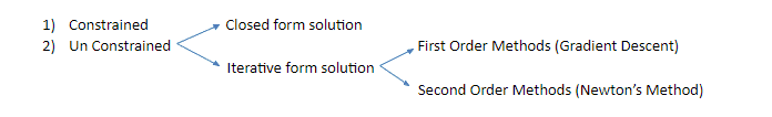
1. Un constrained – Closed Form Solution:

Steepest descent convergence when every element of the gradient is zero (at least very close to zero). In some cases, we may be able to avoid running an iterative algorithm and just jump to the critical point by solving equation  Δxfx=0 for x.

Why is the Iterative method more robust than the closed form?

• Closed form works well for simpler cases, If the cost function has many variables, minimizing using the closed form will be complicated
• Iterative methods will help us reach local minima, most of the time reaching the global minima would be an unaccomplished task.

Gradient Descent (First Order Iterative Method):

Gradient Descent is an iterative method. You start at some Gradient (or) Slope, based on the slope, take a step of the descent. The technique of moving x in small steps with the opposite sign of the derivative is called Gradient Descent. In other words, the positive gradient points direct uphill, and the negative gradient points direct downhill. We can decrease the value off by moving in the direction of the negative gradient. This is known as the method of steepest descent or gradient descent.

New point is proposed by:

Where is the learning rate, a positive scalar determining the size of the step. Choose to a small constant. Popular method to reach with optimum learning rate (ϵ) is by using the grid search or line search.

Choice of Learning Rate:

• Larger learning rate 🡪 Chances of missing the global minima, as the learning curve will show violent oscillations with the cost function increasing significantly.
• Small learning rate 🡪 Convergence is slow and if the learning rate is too low, learning may become stuck with high cost value.

Gradient descent is limited to optimization in continuous spaces, the general concept of repeatedly making a best small move (either positive or negative) toward the better configurations can be generalized to discrete spaces.

Gradient Descent can be associated with the ball rolling down from a valley and the lowest point is the steepest descent, learning rate (ϵ) consider it as the steps taken by the ball to reach the lowest point of the valley.

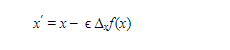
For example, let’s consider the below function as the cost function:

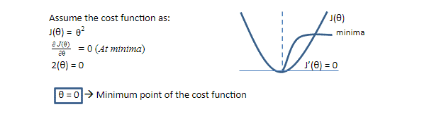
Step by step approach:

1. Start with an initial assumed parameter 🡪 assumed value=(x); = learning rate
2. For the value (x), you calculate the output of the differentiated function which we denote as f’(x)
3. Now, the value of parameter 🡪 x – (ϵ*f'(x))
4. Continue this same process until the algorithm reaches an optimum point (α)
5. Error reduces because the cost function is convex in nature.

The question arises when the derivative function or f’(x) = 0, in that situation the derivative provides no information about which direction to move. Points where f’(x) = 0 are known as critical points or stationary points.

Few other important terminologies to know before we move to SGD:

1. Local Minimum
2. Local Maximum
3. Global Minimum
4. Saddle Points
5. Jacobian Matrix

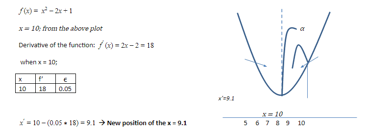
Local Minimum:

Local minimum is a point where f(x) is lower than all neighboring points, so it is no longer possible to decrease f(x) by making baby steps. This is also called as local minima (or) relative minimum.

Local Maximum:

Local Maximum is a point where f(x) is higher than at all neighboring points so it is not possible to increase f(x) by taking baby steps. This is also called a local maxima (or)  relative maximum.

Saddle Points:                                             

Some critical points or stationary points are neither maxima or minima, they are called Saddle points.

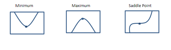
Global Minimum:

Global minimum is the smallest value of the function f(x) that is also called the absolute minimum. There would be only one global minimum whereas there could be more than one or more local minimum. 

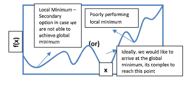
When the input to the function is multidimensional most of the optimization functions fail to find the global minimum as they have multiple local minima, local maxima and saddle points. 

This is one of the greatest challenges in optimization, we often settle with the value of f that is minimal not necessarily global minimum in any formal sense.

What is the Jacobian Matrix?

When we have multiple inputs, we must use partial derivatives of each variable xi. The partial derivative a/axi f(x) measures how f changes as only the variable xi increases at point x. The gradient of f  is the vector containing all the partial derivatives, denoted by xf(x). In multiple dimensions critical points are points where every element of the gradient is equal to zero. 

Sometimes we need to find all derivatives of a function whose input and output are both vectors. The matrix containing all such partial derivatives is known as the Jacobian Matrix. Discussion of Jacobian and Hessian matrices are beyond the scope of current discussion.

Challenges in Gradient Descent:

• For a good generalization we should have a large training set, which comes with a huge computational cost. 
• i.e., as the training set grows to billions of examples, the time taken to take a single gradient step becomes long.

Stochastic Gradient Descent:

Stochastic Gradient Descent is the extension of Gradient Descent.

Any Machine Learning/ Deep Learning function works on the same objective function f(x) to reduce the error and generalize when a new data comes in. 

To overcome the challenges in Gradient Descent we are taking a small set of samples, specifically on each step of the algorithm, we can sample a minibatch drawn uniformly from the training set. The minibatch size is typically chosen to be a relatively small number of examples; it could be from one to few hundred. 

Using the examples from the minibatch. The SGD algorithm then follows the expected gradient downhill:

The Gradient Descent has often been regarded as slow or unreliable, it was not feasible to deal with non-convex optimization problems. Now with Stochastic Gradient Descent, machine learning algorithms work very well when trained, though it reaches the local minimum in the reasonable amount of time. 

A crucial parameter for SGD is the learning rate, it is necessary to decrease the learning rate over time, so we now denote the learning rate at iteration k as Ek.

This brings us to the end of the blog on Stochastic Gradient Descent. We hope that you were able to gain valuable insights about Stochastic Gradient Descent. If you wish to learn more such concepts, enroll with Great Learning Academy’s Free Online Courses and learn now!