When and How to Use Poisson Distribution in Data Analysis

By: Prof. Mukesh Rao (Senior Faculty, Academics, Great Learning)

The Poisson distribution is a discrete probability distribution model that helps quantify events that occur over a specific interval of time, space, or volume. It is particularly useful when analyzing counts, such as defects, website visits, or customer arrivals.

This model represents processes that generate information in the form of counts, i.e., integer values. For example, the number of defects per unit output. The occurrence of a defective piece is an event of interest. The Poisson distribution can be studied on the time axis, in space, or even in volume.

Let’s dive into understanding why the Poisson distribution is used in data analysis.

What is the Poisson Distribution?

Poisson Distribution is a discrete probability distribution. This model represents processes that generate information in counts, i.e., integer values. For example, the number of defects per unit output.

Imagine a chip manufacturing unit. We wish to establish the capability of the process. For this, we gather information from the production line. We collected fifty samples. Those which were defective have a red dot and other not. The occurrence of a defective piece is an event of interest. From now onwards, we will refer to events.

Suppose we observed 25 defective units out of the 50 inspected. Is there a pattern hidden in this data? Or are these defective pieces randomly scattered? If there is a pattern, we can model it and, as discussed earlier, use the model to assess the capability of the process quantitatively. To explore any possible pattern, we analyse the data at a block level instead of individual pieces.

Suppose we pack six output units into one block as shown below. Assuming each output is generated at fixed time interval, each block is six time units long (period).

Poisson distribution can be studied on time axis, space or even volume. In this example, we are analysing it on time axis.

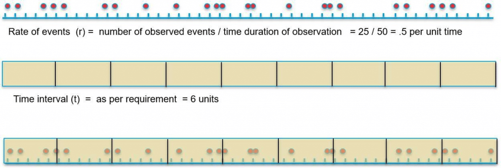
The first observation we can make is, the average number of defectives per time interval (of six units), represented by ʎ is 3. Note: average per time interval is 3 does not mean every time interval will have exactly 3 events.

Variance across time intervals is also 3 (how?). We know ʎ = 3, use the formula for variance, and check out (remember, variance is an average metric, i.e., on average, how much a data point varies from the central value (ʎ) that represents the entire data distribution.

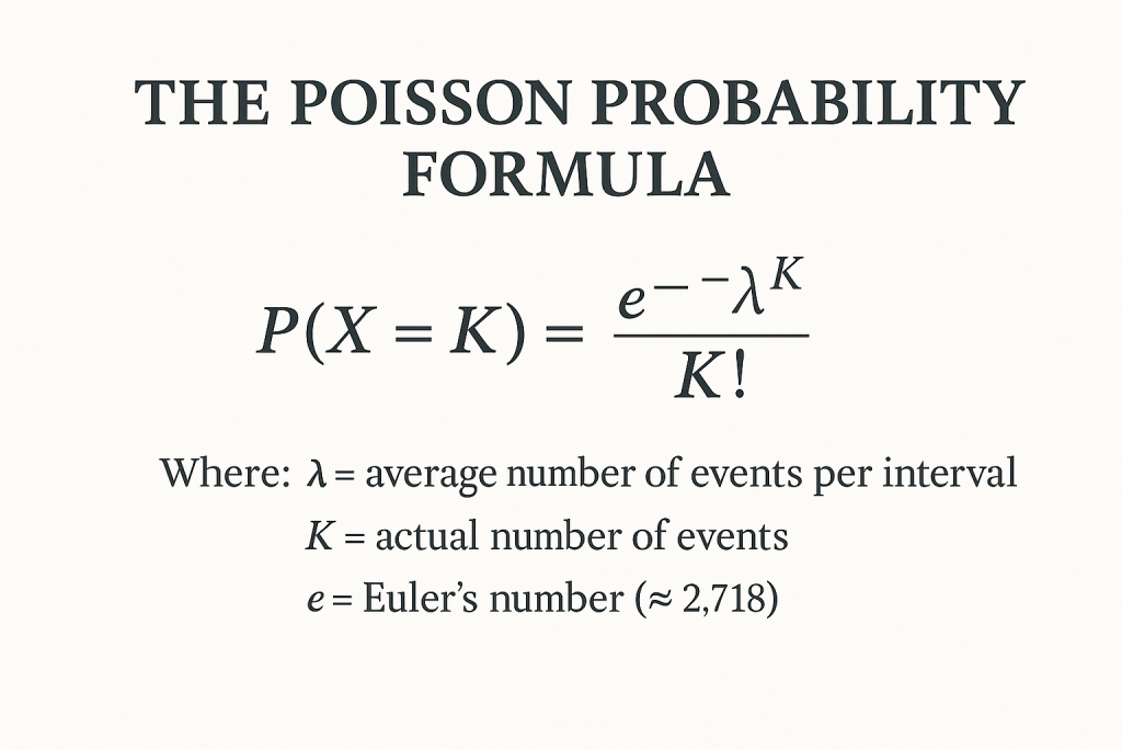
Given the information on the average and variance, we can find the probability of K events per interval using the formula –

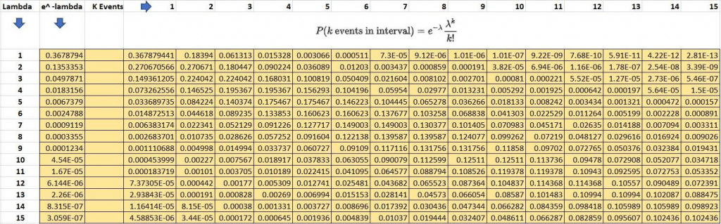
Let us understand this model/formula that represents the Poisson distribution. For that, we have taken different values of ʎ and K and created the following XL grid. This grid is generated for different values of lambda (average number of events per time interval), and for each value of lambda, it shows the probability values of K Events occurring in a time interval

Probability of K Events Observations

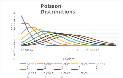
1. In the Poisson distributions graph, each series is for a particular lambda valu,e starting with Series1, which is lambda =1
2. When lambda =1, i.e., the expected number of defects per interval is 1, then the probability of one event per interval, i.e., K=1, will be the highest. As K increases, the probability falls.
3. When lambda = 2 (second row), the expected number of defects per interval is 2 hence, the probability of 2 events per interval i.e., K =2 will be the highest and fall as K increases.
4. The general pattern is – the probability will be highest for that value of K which is equal to the lambda value, and for other values of K for the given lambda, the probability will fall
5. Since this distribution is for positive integers only, for lower values of lambda, the distribution will look asymmetric, but as the value of lambda increases, the distribution tends to become symmetric
6. The function will return smaller and smaller values as ʎ becomes large. When ʎ is large, i.e., the expected number of events in an interval is large, say 10, there are chances of finding events in a large range (1 to 10 and above). Compare this to the case where ʎ = 3, for example, in this case, the range of possible numbers of events less than 3 is small.
7. As a result of point 6, for large values of ʎ, the probability values have to be distributed over a large range; hence, the peak comes down (observe how the peak of the distributions is becoming lower and lower with an increase in ʎ).
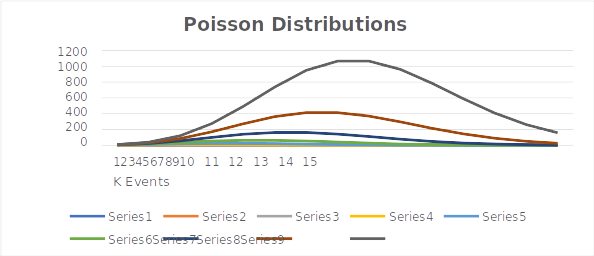
8. What is the role of e^-ʎ? If we do not have the expression e^-ʎin the formula/model, then the numerator will become larger and larger with an increase in lambda, and the result of the calculation will go beyond 1 and thus fail to serve as a probability function
9. Probability of K Events The purpose of e^-ʎis to keep the output in the 0 -1 range to be a valid probability function. Look at the graph below where e^-ʎis removed. The Poisson distribution output is not a probability value

Applications of Poisson Distributions

The Poisson distribution is widely applied in scenarios where discrete events occur randomly but at a known average rate over a fixed interval, be it time, space, distance, or volume. It is particularly powerful when analyzing rare events that are count-based and occur independently of one another.

1. IT & Cybersecurity

• Estimating the number of network intrusions or server failures per day.
• Predicting the number of support tickets raised in a given time period.

2. Sales & E-commerce

• Forecasting the number of units sold per hour/day based on historical averages.
• Estimating the number of transactions or purchases per customer session.

3. Web Analytics & Digital Marketing

• Tracking the number of website visitors or clicks per minute.
• Modeling email open or bounce rates over specific campaigns.

4. Retail & Customer Behavior

• Measuring customer footfall at physical stores per day or per hour.
• Estimating checkout line formation frequency at specific times.

5. Manufacturing & Quality Control

• Calculating the number of defects per production batch.
• Evaluating equipment failure incidents per unit of operational time.

6. Public Health & Transportation

• Modeling the number of disease cases reported per region per week.
• Estimating accidents at intersections or road segments per month.

Why It Matters:

By applying the Poisson distribution in these domains, organizations can:

• Quantify uncertainty with probability,
• Plan resources proactively,
• Reduce downtime or overstaffing,
• Enhance customer satisfaction and operational efficiency.