How to Use the Rank Function & Formula in Excel for Rankings

Ranking data in Excel doesn’t have to be complicated. Whether ranking academic scores or reviewing sales trends, Excel’s RANK function is quite helpful in placing rank positions in your data according to numeric performance. 

However, given the presence of such functions as RANK.EQ and RANK.AVG, it may be challenging to find the most suitable situation for each. 

This tutorial will walk you through learning the basics of the RANK function, how to use it effectively, and give you practical advice on avoiding common mistakes, thus leaving your spreadsheets clean and transparent.

What is the RANK Function in Excel? 

Excel’s RANK function determines the position of a number in a group of numbers. It tells the position of a given number in the sorted sequence of the list. 

The RANK function ranks the top number as 1 by default (descending order), but it can be changed to show a rank increasing when needed. This tool helps to compare values, thus you can rank students in terms of performance or businesses in terms of sales figures.

Syntax and Arguments of the RANK Function 

=RANK(number, ref, [order])

Explanation of each argument:

• Number:
  
  • The number argument is the value whose rank you want to find within a given list or data range.
  • Example: If you want to rank a student’s score, the number would be that student’s score.
    
• Ref:
  • This is the range of numbers against which the number will be ranked.
  • Example: If you have scores of multiple students in cells A1:A10, you would specify this range as A1:A10 to rank the scores relative to the other scores.
    
• Order (optional):
  
  • This argument determines the order of ranking.
  • 0 or omitted: If you leave this argument blank or set it to 0, Excel will rank the numbers in descending order (i.e., the most significant number gets rank 1).
  • Any nonzero value: If you set it to any number other than 0, Excel will rank the numbers in ascending order (i.e., the smallest number gets rank 1).

How To Enter And Apply A Rank Formula In Excel?

1. Enter the Formula in the First Cell
   
   • Click on the cell where you want the formula to appear.
     

Type your formula. For example:

=RANK(A2, $A$2:$A$7, 0)

•  This formula ranks the value in cell A2 within the range A2:A7 in descending order.
  

2. Use the Fill Handle to Copy the Formula
   • After typing the formula, press Enter.
   • Select the cell containing the formula.
   • Hover your mouse over the small square at the bottom-right corner of the selected cell (this is called the fill handle).
   • When the cursor turns into a black cross (+), click and drag the fill handle down or across to the cells where you want to apply the formula.
     
3. Release the Mouse Button
   • Once you’ve highlighted the desired range, release the mouse button.
   • Excel automatically fills the selected cells with the formula, adjusting cell references as needed.
4. Adjusting Formula References (Optional)

If you want to keep specific cell references constant while others change, use absolute references by adding dollar signs ($). For example:

=RANK(A2, $A$2:$A$7, 0)

•  In this formula, $A$2:$A$7 is an absolute reference, meaning it won’t change as you drag the formula.

Tips for Efficient Formula Application

• Double-Click the Fill Handle: Double-click the fill handle if your data range is continuous. Excel will automatically fill the formula with data from the last adjacent cell.
  
• Keyboard Shortcuts:
  
  • Ctrl + D: Fill the formula down in a column.
  • Ctrl + R: Fill the formula to the right in a row.

Master Excel Functions, Formulas & Dashboards with Great Learing Premium course on Excel Training: Beginners to Advanced 

How to Use the RANK Function: Step-by-Step Guide 

Step 1: Prepare Your Data

Ensure you have the data you want to rank in a column. For example, let’s say you have student scores in B2:B7.

Step 2: Decide Where to Display the Rank

You will need to choose where you want to display the rank of each value. For instance, you can display the ranks in column C.

Step 3: Use the RANK Formula

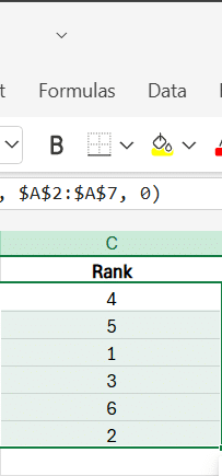
Let’s use the RANK function to assign ranks to each score.

Click on the cell where you want the rank to appear. For example, click on C2 to rank the first score.

Type the following formula:

=RANK(A2, $A$2:$A$6, 0)

• A2: This is the number (score) you want to rank.
• $A$2:$A$6: This is the range of numbers you want to rank against. We use absolute references ($) to keep the range fixed as you drag the formula down.
• 0: This specifies that we want to rank the scores in descending order (highest score gets rank 1).

Step 4: Apply the Formula to Other Cells

After inputting the formula in C2, you can copy it down to automatically rank the data in all other cells of column C.

• Hover your mouse over the small square at the bottom-right corner of the selected cell (C2).
• Drag it down to fill the formula in the rest of the cells, such as C3:C7.

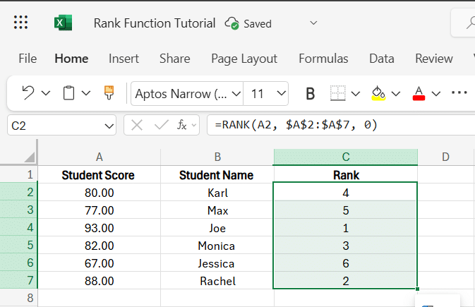
Step 5: Review the Ranks

After applying the formula, you’ll see the ranks next to the corresponding scores.

Step 6: Adjusting for Ties (Optional)

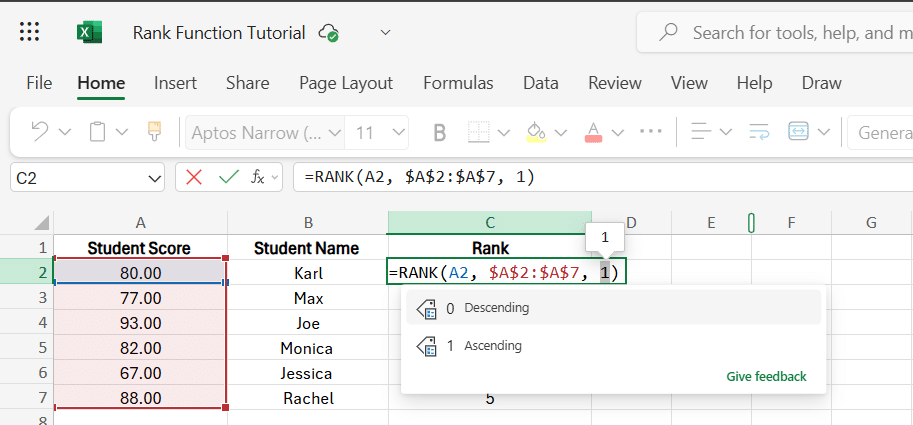
If you prefer to rank the data in ascending order (lower scores get higher ranks), you can change the order argument to 1.

For example, use the formula:

=RANK(A2, $A$2:$A$6, 1)

Step 7: Handle Special Cases (Optional)

If two or more students have such an identical score, the RANK function uses the same position for these students, so it does not move on to the following ranking number.

Additional Tips:

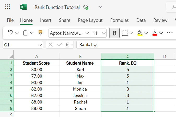
• Use RANK.EQ: If you want to return the same rank for identical numbers, use the RANK.EQ function. It works the same way but explicitly handles ties.

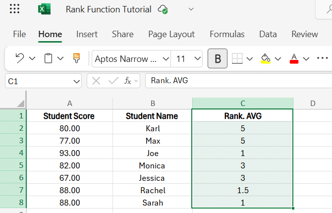
• Use RANK.AVG: If you want the average rank for tied values, use RANK.AVG instead.

Importance Of Using Absolute References To Avoid Formula Errors When Copying

Absolute referencing in formulas for Excel ensures fixed cell references when copying or dragging the formulas to different cells. Such practice is necessary when a steady value, like a tax rate or a multiplier, is applied equally through various formulas.

Example:

Suppose cell B1 contains a fixed tax rate of 5%. To calculate the total price (including tax) for items listed in A2:A10, you would use the formula:

=A2*(1+$B$1)

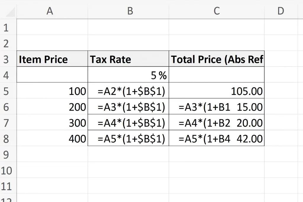
In this example, $B$1 is used as an absolute reference; thus, when the formula is copied from B2 through to B10, it would always look up the tax rate in cell B1, irrespective of the cell movement. If $ signs are not pronounced, the reference will follow the formula and cause calculation errors.

To toggle from relative to absolute references (or vice versa), select the cell reference to change in the formula bar by highlighting it and pressing the F4 key. As each press occurs, you advance through various reference types. ary (e.g., A1), constant (e.g., $A$1), or partly constant (e.g., A$1 or $A1).

Ranking in Ascending vs. Descending Order in Excel

In the RANK function, you can set the order parameter to rank values in a descending order (highest to lowest) or ascending order (lowest to highest).

Descending Order (Default)

• Definition: Ranks the most significant number as 1, followed by the next largest, and so on.
• Use Case: Useful for ranking scores, sales figures, or anything where higher is better.
  

Formula Example:

=RANK(A2, $A$2:$A$10, 0)

• Ranks the value in cell A2 against A2 to A10 in descending order (highest number = rank 1).
  

Ascending Order

• Definition: Ranks the smallest number as 1, followed by the next smallest, and so on.
• Use Case: Useful for ranking race times, expenses, or anything where lower is better.
  

Formula Example:

=RANK(A2, $A$2:$A$10, 1)

• Ranks the value in A2 within A2 to A10 in ascending order (smallest number = rank 1).

Order Type	order Argument	Rank 1 Assigned To	Common Use Cases
Descending (Default)	0 or omitted	Highest value	Scores, revenue, profits
Ascending	1 (or any non-zero)	Lowest value	Times, costs, temperatures

Handling Ties in Rankings (RANK Function in Excel)

When using the RANK function in Excel, duplicate values (ties) are assigned the same rank, and the next rank(s) are skipped to maintain correct rank sequencing.

How Excel Handles Ties:

• If two or more values are equal, they receive the same rank.
• The next rank(s) are skipped accordingly.
  

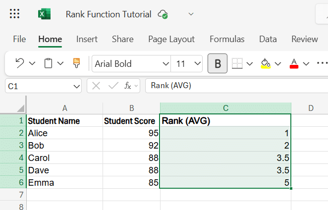
Example:

Explanation:

• Carol and Dave both scored 88, so they share Rank 3.
• Since Rank 3 is assigned twice, Rank 4 is skipped, and Emma’s next rank is 5.

If you want to average the ranks for tied values instead, use RANK.AVG:

=RANK.AVG(B2, $B$2:$B$6, 0)

Advanced Ranking Techniques in Excel

When your dataset contains duplicate values, and you want to assign unique ranks (i.e., no ties), Excel doesn’t handle this natively. Still, with some creativity using functions like COUNTIF and COUNTIFS, you can break ties based on additional logic.

1. Breaking Ties with COUNTIF for Sequential Unique Ranks

This method forces a unique ranking by counting previous occurrences of the same value and adding that count to the rank.

Formula:

=RANK(B3, $B$3:$B$8) + COUNTIF($B$3:B3, B3) – 1

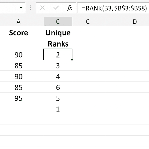
How it works:

• RANK(B3, $B$3:$B$8): Gets the base rank.
• COUNTIF($B$3:B3, B3): Counts how many times the same score has appeared up to the current row.
• Subtracting 1 ensures that only duplicates beyond the first increase the rank.

Result: Tied scores will be ranked sequentially, e.g., 3, 4 instead of both being 3.

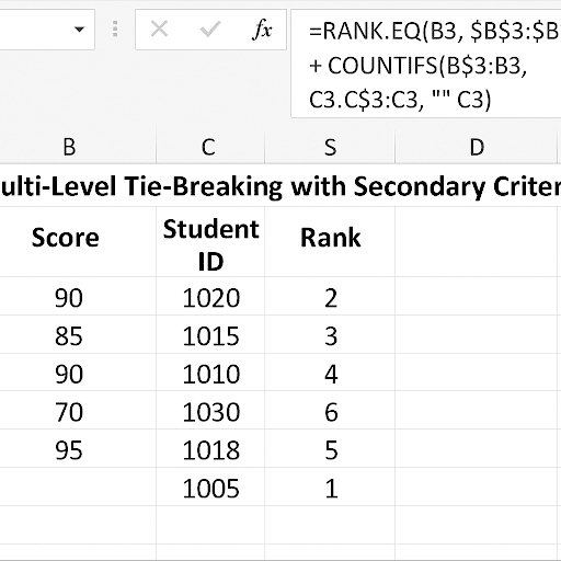
2. Multi-Level Tie-Breaking with Secondary Criteria

If you want to break ties using another column (like timestamp, name, or ID), use RANK.EQ + COUNTIFS.

Example Use-Case: Rank students by score, but if scores are the same, the one with a lower student ID gets the higher rank.

Formula:

=RANK.EQ(B3, $B$3:$B$8) + COUNTIFS(B$3:B3, B3, C$3:C3, “<” & C3)

• B3: Score
• C3: Secondary criterion (e.g., Student ID)
• COUNTIFS(…): Adds +1 for every previous row with the same score but smaller ID, breaking ties.

Technique	Description	Use Case
RANK + COUNTIF	Assigns unique sequential ranks for ties	Simple tie-breaking
RANK.EQ + COUNTIFS	Uses a secondary column to break ties logically	Multi-level sorting (e.g., score + ID)

Common Mistakes and Best Practices When Using the RANK Function in Excel

Common Mistakes

1. Not Using Absolute References ($) in the Range

Mistake:
=RANK(A2, A2:A10)

 When dragged, the range shifts.

Fix:
Use $ to fix the range:

=RANK(A2, $A$2:$A$10)

2. Ignoring Ties in Rankings
   Suppose you’re expecting unique ranks but using plain RANK or RANK.EQ, tied values will produce the same rank, which may not suit all scenarios.
   
3. Using the Wrong Order Argument
   Forgetting the optional third argument can cause incorrect ranking direction.
   
   • 0 or omitted = descending, 1 = ascending.
     
4. Including Non-Numeric Data in the Range
   RANK only works with numbers. Including text or blank cells in the ref range can cause errors or incorrect results.

Best Practices

1. Lock the Range with Absolute References
   
   • Always lock the reference range to prevent it from shifting when dragging the formula.
     
2. Use RANK.EQ or RANK.AVG Where Needed
   
   • RANK.EQ: Gives identical ranks to tied values (default behavior).
   • RANK.AVG: Average ranks for tied values.
     
3. Break Ties with Additional Logic
   
   • Use COUNTIF or COUNTIFS to generate unique ranks when needed (especially for sorted lists or leaderboard applications).
     
4. Double-Check the Order Argument
   
   • Make sure you specify the correct order (ascending vs. descending) based on your ranking logic.
     
5. Test with Edge Cases
   
   • Always test your formula with duplicate, extreme, and empty cells to verify accuracy.

Choosing the Right Ranking Function in Excel: RANK vs RANK.EQ vs RANK.AVG

Function	Description	Ties Handling	Availability	Use Case Example
RANK	Returns the rank of a number in a list.	Assigns the same rank, skips the next rank	Available in all versions	Quick rank of test scores
RANK.EQ	Equivalent to RANK, designed for compatibility with newer Excel versions.	Assigns the same rank, skips the next rank	Excel 2010+	Leaderboards, where equal values share the same rank
RANK.AVG	Returns the average rank for tied numbers.	Assigns average rank	Excel 2010+	Grading systems that require fairness in tie-breaks

Conclusion

Understanding Excel’s ranking functions RANK, RANK.EQ and RANK.AVG helps streamline data analysis for leaderboards, grading systems, or performance metrics. Explore Great Learning’s Data Science and Analytics course to deepen your data analysis skills. The courses will teach you advanced Excel functions and more, empowering you with the skills to tackle real-world data challenges.