Contributed by: Priya Krishnan
LinkedIn Profile: https://www.linkedin.com/in/priya-srinivasan-77b081176/
For all types of Business, whether it is small or large there is a dire need for prediction/estimation. (in terms of Sales, Costs, demand, supply etc). This can be achieved through statistical analysis of underlying data. A probability distribution can be a great tool for such estimations. It has its application in several areas such as Sales Forecasting, Risk Evaluation, Scenario Analysis, etc.
In this article, let us get a brief understanding of Probability Distribution in simple terms. You can also take up the probability for machine learning free online course and learn about the foundations of probability.
Let us start with the basics,
What is Probability? It measures the likelihood of an outcome. Learn about probability and normal distribution with us.
What is an Event? Each possible outcome of a variable is referred to as an event. An event that has no chance of occurring has a probability of 0. (impossible event.) An event that is sure to occur has a probability of 1. (Certain Event)
Example: When we roll an unbiased dice.
Probability of getting a number 5 is an event which is denoted by a Probability P(X=x) function where X represents the actual outcome. x represents one of the possible outcomes. (in this case getting 1/2/3/4/5/6),
P(Y=5)= 1/6= 16.67%
1-> number of ways in which the event occurs
6->total number of possible outcomes
Hence we conclude there is a probability of 16.67% on getting the number 5 by rolling the dice once.
Distribution
The Possible values a variable can take and how frequently they occur
We define distributions using two characteristics only.
- Mean->average value ,
- Variance - what is the spread of the data
On analysing any distribution we need to be sure on two things whether it is a population (all the data) or sample (part of the data)
Notation for Population: Mean = µ, Variance=σ²
Notation for Sample: Mean = x̅, Variance= s2
Since variance is measured in squared units, standard deviation(square root of the variance, For a population – σ, For Sample- S) is preferred a lot for direct interpretation. (That’s why we often encounter µ- σ and µ+σ kind of notations on any normal distribution curve)
Distribution can either be
- narrower and longer – the more congested in the middle of the distribution. The more data falls within the interval (Blue curve in the below Fig)
- or, broader and dispersed - fewer data falls within the interval. The more dispersed the data is. (Red Curve in the below fig)
There is always a constant relationship between mean and variance for any distribution.
Variance equals the expected value of the squared difference from the mean for any value.
σ²=E(X2)- µ2
Before we jump into types of Probability distribution it is essential to know about the types of numeric variables one would encounter on analysing any given data.
Discrete Variables - take values that arise from a counting process.
Continuous Variables - take values that arise from a measuring process.
Based on the type of numeric data, the probability distribution is classified into two types.
i) Discrete Probability Distribution: For a finite number of outcomes- Ex: Roll dice, Picking a Card from a pack of 52 cards.
- Binomial
- Poisson
- HyperGeometric
ii) Continuous Probability Distribution: for Infinitely many outcomes- Ex: Recording time, Distance in Tracking field
- Normal
- Uniform
- Exponential
In general, Each distribution takes this form,
X~N(µ- σ²)
X->Variable
N->Type of Distribution
µ, σ->Characteristics of Distribution
This characteristic varies depending on the type of Distribution.
Discrete Probability Distribution
Bernoulli Distribution:
When there are events with only two possible outcomes (True/False, Success/Failure, 1/0 etc) regardless of one outcome more likely to occur. This is called Binomial with a single trial. (Bern(p)=B(1,p))
For Example:
Imagine a bag of 5 blue and 1 Red ball. Probability of drawing a ball has 2 outcomes.
Getting a red ball or a blue ball. Getting red has the probability of 1/6 and that of the blue ball is 5/6.
How to estimate the Expected Value?
Assigning one outcome as 0 and another outcome as 1
(Generally, the value of interest is assigned 1 and another one is assigned as 0)
Conventionally p>1-p, p as 1 and 0 as 1-p
E(X)= Summation of all possible Outcome values multiplied with their respective Probability values
E(X)=1*p+0*(1-p)=p
E(X)=p
Bernoulli Distribution plot in Python:
Binomial Distribution:
When we carry out the same experiment of (Picking balls from a bag of red and blue balls.) for several iterations then it is Binomial Distribution.
X~B(10,0.6)
Here 10-> number of trials.
0.6-> Probability of one outcome.
What makes Bernoulli and Binomial different?
Imagine a scenario of Surprise quiz test in a classroom. The quiz consists of 10 true/false questions.
- Guessing the answer for one question is a Bernoulli event. Guessing the entire quiz is a Binomial event.
- Expected value of Bernoulli Distribution suggests which outcome is expected out of a single trial. The expected value of Binomial Distribution would suggest the number of times we expect to get a specific outcome. How do we get this? Here comes the Probability Distribution function.
Probability Distribution function
The likelihood of getting a given outcome for a precise number of times.
P(desired outcome)=p
P(alternative outcome)=1-p
There could exist more than one way to reach our desired outcome.
For example, if we wish to find the number of ways to get 2 tail occurrence out of 3 coin flips
TTH,THT,HTT
i.e., 3C2 in mathematical terms. N=3 , x=2
P(x)=(nx).px. (1-p)
Let us take a real time Example of predicting stock price of a single stock of Reliance
Historically you know there is a 60% chance that the stock price will go up and a 40% chance that it will drop.
With probability function, we can calculate the likelihood of stock price increasing 3 times during 5 days.
Here x=3, n=5, p=0.6
After plugging in the formula , we get 34.56%
So we can say, there is a 34.56% likelihood of stock prices increasing 3 times in 5 days time.
Expected value: Sum of all values in the sample space multiplied by their respective probabilities.
E(X)=X0. P(X0)+X1.P(X1)+X2.P(X2)+….XN.P(XN)
X~B(n,p)
E(X)=n.p= 5*0.6=3
σ²=n*p*(1-p)=5*0.6*0.4=1.2
We get, Standard deviation as 1.1
By knowing the expected value and Standard Deviation we can make accurate future forecasts.
Binomial Distribution plot in Python:
Poisson Distribution
It tests how unusual an event frequency is for a given interval
Example: Let us consider a real-time example here.
Scenario: When we need to calculate the number of customers arriving at a bank each minute to plan the number of counters set up.
In this case a customer arriving is an event. The occurrence of each event is independent of one another.
P(X) = (e-μ) (μx) / x!
Find Probability that in a given minute exactly 2 customers arrive,
Plugin x=2, μ=3 in the above formula we get 0.2240 which is 22.40%
The probability that in a given minute more than 2 customers arrive,
P(X>2)=1-P(X<=2) We get, 0.5768 which is 57.68%
Thus, we conclude there is a 57.68% chance that more than 2 customers will arrive at the same minute.
Poisson Distribution plot in Python:
Hypergeometric Distribution
It is a binomial distribution without replacement. The outcome of each trial is dependent on each other.
Imagine we have a population of N items which consist of 2 categories.
‘Category 1’ with k items and ‘Category 2’ with N-k items.
n items are chosen at random which will again contain 2 categories of items. Let Category 1 be x and Category 2 be n-x then the probability function is given as,
P(X)=kcx * (N-k)C(n-x) / NCn
Example: To find the probability of choosing 2 items from a population size of 100 items which contains 20 ‘Category 1’ items and 80 ‘Category 2’ items.
When we plug these values N=100 , k=20, N-k=80, n=2 in the above formula, Probability of both the items to belong to ‘Category1’ alone is, 19/495=0.0383 which is 3.83%
Hypergeometric Distribution plot in Python:
Continuous Probability Distribution
The distribution would be a curve and not disconnected bars because here we consider continuous outcomes of an experiment. Probability Density Function is a mathematical expression that defines the distribution of the values for a continuous variable.
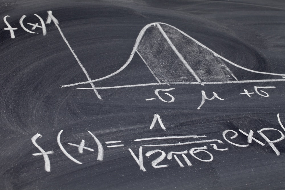
Normal Distribution
The outcome of many distributions in nature closely resembles this distribution. (Simple Example: height, weight, blood pressure of Human Being) Hence the name normal. It is symmetrical and bell-shaped implying that most observed values tend to cluster around the mean. Although the values range from negative infinity to positive infinity. Extreme small or Extreme large values are very unlikely to occur.
Sample plot:
Probability Function: X~N(µ,σ²)
Most of the Statistical Analysis assumes the data to be normally distributed. We can standardise the data to fit in between 0 and 1 (by means of applying any operators like addition, subtraction, multiplication, division) without affecting the type of distribution. This is called Transformation.
(Z=x- µ/ σ)
Normal Distribution plot In Python:
Uniform Distribution
All outcomes of this event are equally likely. They are said to be equ-probable. These outcomes tend to follow a uniform distribution. These are also called Rectangular Distribution. It is symmetrical therefore the mean is equal to the median. It can be both discrete and continuous.
X~U(a,b) (in the below example, it is -a to +a)
a->start Value, b->End value
Sample plot:
Expected value(mean) provides no relevant information because all outcomes have the same probability value. Since there is no variation, there is no predictive power.
Uniform Distribution plot in Python:
Exponential Distribution
Events that are rapidly changing take this distribution.
Example: Online news that gets generated each second.
This is skewed to the right making the mean larger than median. Range is from 0 to positive infinity.
Distribution shape makes it unlikely that extremely large values will occur.
Sample plot:
Exponential Distribution plot in Python:
To Summarize…
In this article, we discussed the basics of Probability, Probability Distribution, and its types, and how to generate various distribution plots in Python. So, if you are someone who chooses to get into a Data Science journey, it is imperative to get a hold of Probability concepts to solve complex business problems.
To learn about more concepts and pursue a career in Data Science, upskill with Great Learning's PG program in Data Science and Engineering. (Now this program has become Data Science Course with Gen AI program)