Hill Climbing Algorithm in Artificial Intelligence

Hill Climbing Algorithm
Working Process
Types of Hill Climbing
State Space Concept for Hill Climbing
Problems faced in Hill Climbing Algorithm
Case Study

Introduction

There are diverse topics in the field of Artificial Intelligence and Machine learning. Research is required to find optimal solutions in this field. In Deep learning, various neural networks are used but optimization has been a very important step to find out the best solution for a good model. In the field of AI, many complex algorithms have been used. It is also important to find out an optimal solution. Hill climbing algorithm is one such optimization algorithm used in the field of Artificial Intelligence. It is a mathematical method which optimizes only the neighboring points and is considered to be heuristic. A heuristic method is one of those methods which does not guarantee the best optimal solution. This algorithm belongs to the local search family. Now let us discuss the concept of local search algorithms.

Working Process

This algorithm works on the following steps in order to find an optimal solution.

It tries to define the current state as the state of starting or the initial state.
It generalizes the solution to the current state and tries to find an optimal solution. The solution obtained may not be the best.
It compares the solution which is generated to the final state also known as the goal state.
It will check whether the final state is achieved or not. If not achieved, it will try to find another solution.

Types of Hill Climbing

There are various types of Hill Climbing which are-

Simple Hill climbing
Steepest-Ascent Hill climbing
Stochastic Hill climbing

Simple Hill Climbing

Simple Hill Climbing is one of the easiest methods. It performs evaluation taking one state of a neighbor node at a time, looks into the current cost and declares its current state. It tries to check the status of the next neighbor state. If it finds the rate of success more than the previous state, it tries to move or else it stays in the same position. It is advantageous as it consumes less time but it does not guarantee the best optimal solution as it gets affected by the local optima.

Algorithm:

Step 1: It will evaluate the initial state.

Condition:
a) If it is found to be final state, stop and return success
b) If it is not found to be the final state, make it a current state.

Step 2: If no state is found giving a solution, perform looping.

A state which is not applied should be selected as the current state and with the help of this state, produce a new state.
Evaluate the new state produced.

Conditions:
1. If it is found to be final state, stop and return success.
2. If it is found better compared to current state, then declare itself as a current state and proceed.
3. If it is not better, perform looping until it reaches a solution.

Step3: Exit the process.

Steepest Ascent Hill climbing

This algorithm selects the next node by performing an evaluation of all the neighbor nodes. The node that gives the best solution is selected as the next node.

Algorithm:

Step 1: Perform evaluation on the initial state.

Condition:
a) If it reaches the goal state, stop the process
b) If it fails to reach the final state, the current state should be declared as the initial state.

Step 2: Repeat the state if the current state fails to change or a solution is found.

Step 3: Exit

Stochastic Hill Climbing

This algorithm is different from the other two algorithms, as it selects neighbor nodes randomly and makes a decision to move or choose another randomly. This algorithm is very less used compared to the other two algorithms.

Features:

The features of this algorithm are given below:

It uses a greedy approach as it goes on finding those states which are capable of reducing the cost function irrespective of any direction.
It is considered as a variant in generating expected solutions and the test algorithm. It first tries to generate solutions that are optimal and evaluates whether it is expected or not. If it is found the same as expected, it stops; else it again goes to find a solution.
It does not perform a backtracking approach because it does not contain a memory to remember the previous space.

Also check: Backtracking Algorithm

State Space Concept for Hill Climbing

A state space is a landscape or a region which describes the relation between cost function and various algorithms. The following diagram gives the description of various regions.

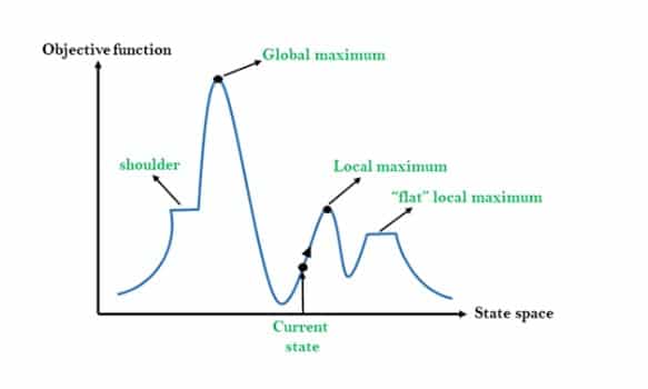
Local Maximum: As visible from the diagram, it is the state which is slightly better than the neighbor states but it is always lower than the highest state.

Global maximum: It is the highest state of the state space and has the highest value of cost function.

Current State: It is the state which contains the presence of an active agent.

Flat local maximum: If the neighbor states all having same value, they can be represented by a flat space
(as seen from the diagram) which are known as flat local maximums.

Shoulder region: It is a region having an edge upwards and it is also considered as one of the problems in hill climbing algorithms.

Problems faced in Hill Climbing Algorithm

Local maximum: The hill climbing algorithm always finds a state which is the best but it ends in a local maximum because neighboring states have worse values compared to the current state and hill climbing algorithms tend to terminate as it follows a greedy approach.

To overcome such problems, backtracking technique can be used where the algorithm needs to remember the values of every state it visited.

Plateau: In this region, all neighbors seem to contain the same value which makes it difficult to choose a proper direction.

To overcome such issues, the algorithm can follow a stochastic process where it chooses a random state far from the current state. That solution can also lead an agent to fall into a non-plateau region.

Ridge: In this type of state, the algorithm tends to terminate itself; it resembles a peak but the movement tends to be possibly downward in all directions.

To overcome such issues, we can apply several evaluation techniques such as travelling in all possible directions at a time.

Applications of Hill climbing technique

Robotics

Hill climbing Is mostly used in robotics which helps their system to work as a team and maintain coordination.

Marketing

The algorithm can be helpful in team management in various marketing domains where hill climbing can be used to find an optimal solution. The travelling time taken by a sale member or the place he visited per day can be optimized using this algorithm.

Case Study

We will perform a simple study in Hill Climbing on a greeting “Hello World!”. We will see how the hill climbing algorithm works on this. Though it is a simple implementation, still we can grasp an idea how it works.

First, we will import all the libraries.

import random
import string

We will generate random solutions and evaluate our solution. If the solution is the best one, our algorithm stops; else it will move forward to the next step.

#random solution generates
def random_solution(length=13):
    return [random.choice(string.printable) for _ in range(length)]

#evaluate a solution
def evaluate_sol(solution):
    target = list ("Hello, World!")
    diff = 0
    for i in range(len(target)):
        s = solution[i]
        t = target[i]
        diff += abs(ord(s) - ord(t))
    return diff

Now we will try mutating the solution we generated. It is mostly used in genetic algorithms, and it means it will try to change one of the letters present in the string “Hello World!” until a solution is found.

#mutating a solution
def mutate_sol(solution):
    index = random.randint(0, len(solution) - 1)
    solution[index] = random.choice(string.printable)

Now we will try to generate the best solution defining all the functions. Let’s see how it works after putting it all together.

best = random_solution()
best_score = evaluate_sol(best)

while True:
    print ('Best score so far', best_score, 'Solution', "“. join(best))

    if best_score == 0:
        break

    new_solution = list(best)
    mutate_sol(new_solution)



    score = evaluate_sol(new_solution)
    if evaluate_sol(new_solution) < best_score:
        best = new_solution
        best_score = score

After running the above code, we get the following output.

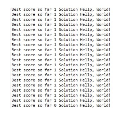
As we can see first the algorithm generated each letter and found the word to be “Hello, World!”. It tried to generate until it came to find the best solution which is “Hello, World!”. So, it worked.

This algorithm is less used in complex algorithms because if it reaches local optima and if it finds the best solution, it terminates itself. It also does not remember the previous states which can lead us to problems. To avoid such problems, we can use repeated or iterated local search in order to achieve global optima. Other algorithms like Tabu search or simulated annealing are used for complex algorithms.

If you found this helpful and wish to learn more, check out Great Learning’s course on Artificial Intelligence and Machine Learning today.