Artificial Intelligence and Machine Learning are transforming the world. AI-ML leads almost every sector, from driving innovation to making processes smarter and delivering personalized experiences.
At the core of this technology, we have a strong computational framework known as Neural Networks, which mimics how the human brain works. It has the ability to learn from data. To learn more about Neural Networks, check out our blog, Definition and Types of Neural Networks.
The backpropagation algorithm is one of the most crucial aspects that make this ability to learn possible. It is an algorithm that trains neural networks to perform complex tasks like recognizing patterns, translating languages, and diagnosing diseases.
In this blog, we will have a complete understanding of this algorithm and the importance of the backpropagation algorithm in machine learning. To deepen your knowledge of machine learning, this algorithm is a must-know concept.
What is Backpropagation?
Backpropagation is a short form of backward propagation of errors. It is the key that unlocks the learning potential of neural networks. It is the practice of perfectly tuning the weights of neural networks based on the Loss, known as the error rate, obtained in iteration.
It plays a fundamental role in neural networks by:
- Identifying Errors: Measuring the difference between a network's prediction and the actual result.
- Providing Feedback: Calculate the network layer that indulged in the error.
- Correcting Mistakes: To minimize errors in future, it adjusts the weights and biases.
Backpropagation allows neural networks to achieve better performance and high accuracy. It is mainly preferred to adapt and generalize new data.
Significance of Backpropagation
Backpropagation's ability to modify deep learning algorithms by efficiently training neural networks for various complexities stands out among all the algorithms.
- Efficiency in training: This algorithm allows the network to measure gradients layer by layer, which reduces computational costs on a larger scale.
- Flexibility: It is versatile across domains as it supports different loss functions, activation functions and optimization techniques.
- Scalability: It enables the efficient training of architectures with hundreds of layers.
Common examples of backpropagation are breakthroughs in natural language processing like GPT models and computer vision like facial recognition.
Steps of the Backpropagation Algorithm
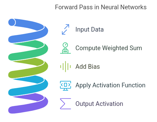
1. Forward Pass
To understand the backpropagation algorithm step by step, we first need to understand the concept of forward pass. This is the process where predictions are made after passing the data through the network.
The three types of layers are:
- Input Layer: The data enters the network in this layer. For example, the input could be pixel values if the task is facial recognition.
- Hidden Layers: In these layers, the data is transformed based on weights, biases and activation functions.
- Output Layer: The network produces a prediction in this layer. Authenticating the biometrics of the face in the above example.
Formula of Forward pass:
Compute activations (a) using weights (W), biases (b), and inputs (x):

z=W⋅x+b and a=f(z)

Here, f(z) is the activation function (e.g., sigmoid, ReLU).
To learn more about the activation functions that help transform data in hidden layers, check out our article What are Activation Functions in Neural Networks?
2. Error Calculation
This is the step of measuring mistakes. The network evaluates how far off the prediction matches the actual answer in this step. This is done by using a loss function, which can be:
- Mean Squared Error(MSE) for regression tasks.
- Cross-entropy Loss for classification tasks.
3. Backward Pass
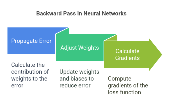
This is the step where backpropagation works. It has two functions:
- Propagating the error: The algorithm calculates how much weight in the network layers contributed to the error.
- Adjusting the weights: Using the above information, the weights and biases are adjusted to reduce the error for the next iteration.
Weights and biases are adjusted using gradient descent:
Weight new = Weightold - Gradient

Here, η is the learning rate, a parameter that controls the step size for updates.

Backward Pass: Calculate gradients of the loss function (LLL) concerning weights using the chain rule:

          LW=LaazzW
This tells us how much to adjust W.
Repeat: Iterate the above process for multiple cycles for the entire dataset until the network achieves targeted results.
Python code for step-by-step implementation:
# Training loop

epochs = 10000

for epoch in range(epochs):

# Forward pass

hidden_layer_input = np.dot(inputs, weights_input_hidden) + bias_hidden

hidden_layer_output = sigmoid(hidden_layer_input)

output_layer_input = np.dot(hidden_layer_output, weights_hidden_output) + bias_output

predicted_output = sigmoid(output_layer_input)

# Backward pass

error = targets - predicted_output

d_predicted_output = error * sigmoid_derivative(predicted_output)

error_hidden_layer = d_predicted_output.dot(weights_hidden_output.T)

d_hidden_layer = error_hidden_layer * sigmoid_derivative(hidden_layer_output)

# Update weights and biases

weights_hidden_output += hidden_layer_output.T.dot(d_predicted_output) * learning_rate

weights_input_hidden += inputs.T.dot(d_hidden_layer) * learning_rate

bias_output += np.sum(d_predicted_output, axis=0, keepdims=True) * learning_rate

bias_hidden += np.sum(d_hidden_layer, axis=0, keepdims=True) * learning_rate

# Print loss at intervals

if epoch % 1000 == 0:

loss = mean_squared_error(targets, predicted_output)

print(f"Epoch {epoch}, Loss: {loss:.4f}")
Code Explanation
1. Forward Pass:
- Hidden Layer: Computes hidden_input= XW + b then applies the sigmoid activation.
- Output Layer: Computes output_input= HW + b, followed by sigmoid for predictions.
Backward Pass (Error Propagation):
- Output Layer Error:
error = targets - predicted_output
Gradient: doutput= error x sigmoid_derivative.
- Hidden Layer Error: Propagates error backwards and computes gradients.
Weights and Bias Updates:
- Adjust weights and biases using the gradients and learning rate.
Monitor Loss:
- Every 1000 epochs, it calculates and prints the Loss (mean squared error).
Real-World Applications
Backpropagation in machine learning is used in the following ways:
- Natural Language Processing: Performing tasks like translation and sentiment analysis with backpropagation algorithms is easier.
- Image Recognition: Neural networks trained with this algorithm identify objects in photos.
- Self-driving Cars: The algorithm trains systems to sense traffic signs and obstacles.
Challenges in Backpropagation
Backpropagation is one of the most potent algorithms of machine learning, yet it has some challenges, such as:
- Vanishing gradients: In complex networks, sometimes gradients become too small to update weights effectively.
- Exploding gradients: Conversely, gradients sometimes become too large, destabilizing training.
- Computational intensity: Specific computational resources are required to train deep networks, which may be costly.
Various optimization techniques can help backpropagation overcome these challenges, such as gradient clipping, batch normalization techniques, or advanced optimizer algorithms such as Adam and RMSProp.
Suggest Read: What is Gradient Boosting?
To understand the challenges of vanishing gradients in deep learning, learn more about this problem in our article What is Vanishing Gradient Problem?
Learn Backpropagation Hands-on
Enthusiastic in learning backpropagation real-life working? You can enrol in the Free Machine Learning Course, which offers in-depth tutorials on backpropagation algorithms and other essential deep-learning topics.
For tech enthusiasts, we provide Artificial Intelligence and Machine Learning courses that offer in-depth knowledge of AI-ML along with practical experience.
Also, you can enroll in a Free Python Course to use Python scripts in tools like Tensorflow and Pytorch to conduct practical experiments with this algorithm.
Conclusion
The backpropagation algorithm acts as a key in neural network training. Iteratively adjusting weights and biases helps models achieve greater accuracy. Whether you are a beginner or a professional, this blog provides in-depth information about backpropagation algorithms and their usage in machine learning. This technology empowers your machine-learning skills and enables your data to learn and improve.
Suggested Read: Backpropagation through time - RNN