Whether predicting the next word within a sentence or identifying trends in financial markets, the capacity to interpret and analyze sequential data is vital in today’s AI world.
The traditional neural networks often fail at learning long-term patterns. Enter LSTM (Long Short-Term Memory), a specific recurrent neural network that changed how machines operate with time-dependent data.
In this article, we’ll explore in depth how LSTM works, its architecture, the decoding algorithm used, and how it is helping solve real-world problems across industries.
Understanding LSTM
Long Short-Term Memory (LSTM) is a type of Recurrent Neural Network (RNN) that addresses the shortcomings of standard RNNs in terms of their capacity to track long-term dependencies, which is a result of their vanishing or exploding gradients.
Invented by Sepp Hochreiter and Jürgen Schmidhuber, the LSTM presented an architecture breakthrough using memory cells and gate mechanisms (input, output, and forget gates), allowing the model to retain or forget information across time, 1997, selectively.
This invention was especially effective for sequential purposes such as speech recognition, language modeling, and time series forecasting, where understanding the context throughout time is a significant factor.
LSTM Architecture: Components and Design
Overview of LSTM as an Advanced RNN with Added Complexity
Although traditional Recurrent Neural Networks (RNNs) can process serial data, they cannot handle long-term dependencies because of their related gradient problem.
LSTM (Long Short-Term Memory) networks are an extension of RNNs, with a more complex architecture to help the network learn what to remember, what to forget, and what to output over more extended sequences.
This level of complexity makes LSTM superior in deep context-dependent tasks.
Core Components
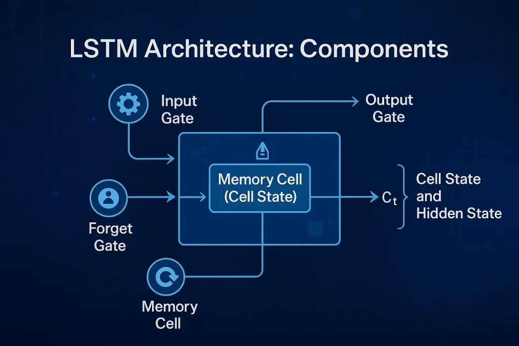
- Memory Cell (Cell State):
The memory cell is the epicenter of the LSTM unit. A conveyor belt transports information across time steps with minimal alterations. The memory cell allows LSTM to store information for long intervals, making it feasible to capture long-term dependencies.
- Input Gate:
The input gate controls the entry into the memory cell of new information. It applies a sigmoid activation function to determine which values will be updated and a tanh function to generate a candidate vector. This gate makes it possible to store only relevant new information.
- Forget Gate:
This gate determines what should be thrown out of the memory cell. It gives values between 0 and 1; 0: “completely forget”, 1: “completely keep”. This selective forgetting is essential in avoiding memory overload.
- Output Gate:
The output gate decides what piece in the memory cell goes to the next hidden state (and maybe even as output). It supports the network in determining which information from the current cell state would influence the next step along the sequence.
Cell State and Hidden State:
- Cell State (C<sub>t</sub>): It carries long-term memory modified by input and forget gates.
- Hidden State (h<sub>t</sub>): Represents the output value of the LSTM unit in a particular time step, which depends upon both the cell state and the output gate. It is transferred to the next LSTM unit and tends to be used in the final prediction.
Certificate Program in Applied Generative AI
Master the tools and techniques behind generative AI with expert-led, project-based training from Johns Hopkins University.
How do These Components Work Together?
The LSTM unit performs the sequence of operations in every time step:
- Forget: The forget gate uses the previous hidden state and current input to determine information to forget from the cell state.
- Input: The input gate and the candidate values determine what new information needs to be added to the cell state.
- Update: The cell state is updated when old retention information is merged with the chosen new input.
- Output: The output gate will use the updated cell state to produce the next hidden state that will control the next step, and might be the output itself.
This complex gating system enables LSTMs to keep a well-balanced memory, which can retain critical patterns and forget unnecessary noise that traditional RNNs find difficult.
LSTM Algorithm: How It Works
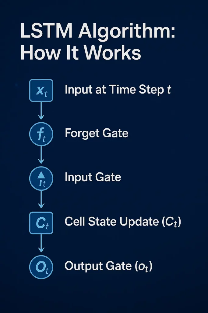
- Input at Time Step :
At each time step ttt, the LSTM receives two pieces of information:
- xtx_txt: The current input to the LSTM unit (e.g., the next word in a sentence, or the next time value in a sequence
- ht−1h_{t-1}ht−1: The previous hidden state carries the prior time step information.
- Ct−1C_{t-1}Ct−1: The previous cell state carries long-term memory from prior time steps.
- Forget Gate (ftf_tft):
The forget gate decides what information from the previous cell state should be discarded. It looks at the current input xtx_txt and the last hidden state ht−1h_{t-1}ht−1 and applies a sigmoid function to generate values between 0 and 1. 0 means “forget completely,” and 1 means “keep all information.”
- Formula:

Where σ\sigmaσ is the sigmoid function, WfW_fWf is the weight matrix, and bfb_fbf is the bias term.
- Formula:
- Input Gate (iti_tit):
The input gate determines what new information should be added to the cell state. It has two components:
- The sigmoid layer decides which values will be updated (output between 0 and 1).
- The tanh layer generates candidate values for new information.
- Formula:

Where C~t\tilde{C}_tC~t is the candidate cell state, and WiW_iWi, WCW_CWC are weight matrices for the input gate and cell candidate, respectively.
- Cell State Update (CtC_tCt):
The cell state is updated by combining the previous Ct−1C_{t-1}Ct−1 (modified by the forget gate) and the new information generated by the input gate. The forget gate’s output controls how much of the previous cell state is kept, while the input gate’s output controls how much new information is added.
- Formula:

- ftf_tft controls how much of the previous memory is kept,
- iti_tit decides how much of the new memory is added.
- Formula:
- Output Gate (oto_tot):
The output gate determines which information from the cell state should be output as the hidden state for the current time step.


The current input xtx_txt and the previous hidden state ht−1h_{t-1}ht−1 are passed through a sigmoid function to decide which parts of the cell state will influence the secret state. The tanh function is then applied to the cell state to scale the output.
- Formula:

WoW_oWo is the weight matrix for the output gate, bob_obo is the bias term, and hth_tht is the hidden state output at time step ttt.

Mathematical Equations for Gates and State Updates in LSTM
- Forget Gate (ftf_tft):
The forget gate decides which information from the previous cell state should be discarded. It outputs a value between 0 and 1 for each number in the cell state, where 0 means "completely forget" and 1 means "keep all information."
Formula-

- σ\sigmaσ: Sigmoid activation function
- WfW_fWf: Weight matrix for forget gate
- bfb_fbf: Bias term
- Input Gate (iti_tit):
The input gate controls what new information is stored in the cell state. It decides which values to update and applies a tanh function to generate a candidate for the latest memory.
Formula-

- C~t\tilde{C}_tC~t: Candidate cell state (new potential memory)
- tanh\tanhtanh: Hyperbolic tangent activation function
- Wi, WCW_i, W_CWi, WC: Weight matrices for input gate and candidate cell state
- bi,bCb_i, b_Cbi,bC: Bias terms
- Cell State Update (CtC_tCt):
The cell state is updated by combining the information from the previous cell state and the newly selected values. The forget gate decides how much of the last state is kept, and the input gate controls how much new information is added.
Formula-

- Ct−1C_{t-1}Ct−1: Previous cell state
- ftf_tft: Forget gate output (decides retention from the past)
- iti_tit: Input gate output (decides new information)
- Output Gate (oto_tot):
The output gate determines what part of the cell state should be output at the current time step. It regulates the hidden state (hth_tht) and what information flows forward to the next LSTM unit.
Formula- ![]()
- Hidden State (hth_tht):
The hidden state is the LSTM cell output, which is often used for the next time step and often as the final prediction output. The output gate and the current cell state determine it.
Formula- ![]()
- hth_tht: Hidden state output at time step ttt
- oto_tot: Output gate’s decision
PG Program in AI & Machine Learning
Master AI with hands-on projects, expert mentorship, and a prestigious certificate from UT Austin and Great Lakes Executive Learning.
Comparison: LSTM vs Vanilla RNN Cell Operations
| Feature | Vanilla RNN | LSTM |
| Memory Mechanism | Single hidden state vector hth_tht | Dual memory: Cell state CtC_tCt + Hidden state hth_tht |
| Gate Mechanism | No explicit gates to control information flow | Multiple gates (forget, input, output) to control memory and information flow |
| Handling Long-Term Dependencies | Struggles with vanishing gradients over long sequences | Can effectively capture long-term dependencies due to memory cells and gating mechanisms |
| Vanishing Gradient Problem | Significant, especially in long sequences | Mitigated by cell state and gates, making LSTMs more stable in training |
| Update Process | The hidden state is updated directly with a simple formula | The cell state and hidden state are updated through complex gate interactions, making learning more selective and controlled |
| Memory Management | No specific memory retention process | Explicit memory control: forget gate to discard, input gate to store new data |
| Output Calculation | Direct output from hth_tht | Output from the oto_tot gate controls how much the memory state influences the output. |
Training LSTM Networks
1. Data Preparation for Sequential Tasks
Proper data preprocessing is crucial for LSTM performance:
- Sequence Padding: Ensure all input sequences have the same length by padding shorter sequences with zeros.
- Normalization: Scale numerical features to a standard range (e.g., 0 to 1) to improve convergence speed and stability.
- Time Windowing: For time series forecasting, create sliding windows of input-output pairs to train the model on temporal patterns.
- Train-Test Split: Divide the dataset into training, validation, and test sets, maintaining the temporal order to prevent data leakage.
2. Model Configuration: Layers, Hyperparameters, and Initialization
- Layer Design: Begin with an LSTM layer [1] and finish with a Dense output layer. For complex tasks, layer stacking LSTM layers can be considered.
- Hyperparameters:
- Learning Rate: Start with a value from 1e-4 to 1e-2.
- Batch Size: Common choices are 32, 64, or 128.
- Number of Units: Usually between 50 and 200 units per LSTM layer.
- Dropout Rate: Dropout (e.g., 0.2 to 0.5) can solve overfitting.
- Weight Initialization: Use Glorot or He initialization of weights to initialize the initial weights to move faster towards convergence and reduce vanishing/exploding gradient risks.
3. Training Process
Knowing the basic elements of LSTM training
- Backpropagation Through Time (BPTT)- This algorithm calculates gradients by unrolling the LSTM over time to allow the model to learn sequential dependencies.
- Gradient Clipping: Clip backpropagator- gradients during backpropagation to a given threshold (5.0) to avoid exploding gradients. This helps in the stabilization of training, especially in deep networks.
- Optimization Algorithms- Optimizer can be chosen to be of Adam or RMSprop type, which adjust their learning rates and are suitable for training LSTM.
Applications of LSTM in Deep Learning
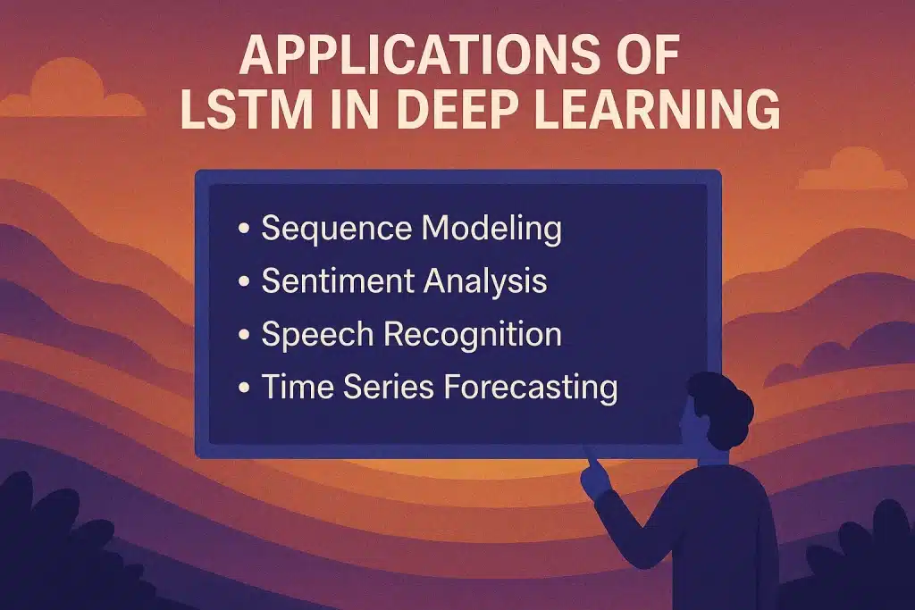
1. Time Series Forecasting
Application: LSTM networks are common in time series forecasting, for ex. Forecasting of stock prices, weather conditions, or sales data.
Why LSTM?
LSTMs are highly effective in capturing such long-term dependencies and trends in sequential data, making LSTMs excellent in forecasting future values based on previous ones.
2. Natural Language Processing (NLP)
Application: LSTMs are well used in such NLP problems as machine translation, sentiment analysis, and language modelling.
Why LSTM?
LSTM’s confluence in remembering contextual information over long sequences enables it to understand the meaning of words or sentences by referring to surrounding words, thereby enhancing language understanding and generation.
3. Speech Recognition
Application: LSTMs are integral to speech-to-text, which converts spoken words to text.
Why LSTM?
Speech has temporal dependency, with words spoken at earlier stages affecting those spoken later. LSTMs are highly accurate in sequential processes, successfully capturing the dependency.
4. Anomaly Detection in Sequential Data
Application: LSTMs can detect anomalies in data streams, such as fraud detection when financial transactions are involved or malfunctioning sensors in IoT networks.
Why LSTM?
With the learned Normal Patterns of Sequential data, the LSTMs can easily identify new data points that do not follow the learned patterns, which point to possible Anomalies.
5. Video Processing and Action Recognition
Application: LSTMs are used in video analysis tasks such as identifying human actions (e.g, walking, running, jumping) based on a sequence of frames in a video (action recognition).
Why LSTM?
Videos are frames with temporal dependencies. LSTMs can process these sequences and are trained to learn over time, making them useful for video classification tasks.
Conclusion
LSTM networks are crucial for solving intricate problems in sequential data coming from different domains, including but not limited to natural language processing and time series forecasting.
To take your proficiency a notch higher and keep ahead of the rapidly growing AI world, explore the Post Graduate Program in Artificial Intelligence and Machine Learning being provided by Great Learning.
This integrated course, which was developed in partnership with the McCombs School of Business at The University of Texas at Austin, involves in-depth knowledge on topics such as NLP, Generative AI, and Deep Learning.
With hands-on projects, live mentorship from industry experts, and dual certification, it is intended to prepare you with the skills necessary to do well in AI and ML jobs.