- What is NumPy in Python?
- How to install NumPy Python?
- NumPy Creating Arrays
- Operations using NumPy
- NumPy - Data Types
- Data Type Objects (dtype)
- ndarray.shape
- ndarray.ndim
- numpy.itemsize
- numpy.flags
- NumPy - Array Creation Routines
- numpy.zeros
- NumPy - Indexing & Slicing
- NumPy - Advanced Indexing
- Integer Indexing
- Boolean Array Indexing
- NumPy - Broadcasting
- NumPy - Iterating Over Array
- NumPy - Array Manipulation
- NumPy - Mathematical Functions
- NumPy - Byte Swapping
- NumPy - Copies & Views
- numpy.matlib.eye()
- NumPy - Matplotlib
- NumPy - Using Matplotlib
- numpy.save()
- NumPy Array Join
- NumPy Array Split
- Split into Arrays
- Arithmetic
- Frequently Asked Questions on NumPy in Python
So you've learned the basics of Python and you're looking for a more powerful way to analyse data? NumPy is what you need.NumPy is a module for Python that allows you to work with multidimensional arrays and matrices. It's perfect for scientific or mathematical calculations because it's fast and efficient. In addition, NumPy includes support for signal processing and linear algebra operations. So if you need to do any mathematical operations on your data, NumPy is probably the library for you.
In this tutorial, we'll show you how to use NumPy to its full potential. You'll learn more about arrays as well as operate on them using mathematical functions.
In this course, you will learn the fundamentals of Python: from basic syntax to mastering data structures, loops, and functions. You will also explore OOP concepts and objects to build robust programs.
NumPy, which stands for Numerical Python, is a library consisting of multidimensional array objects and a collection of routines for processing those arrays. Using NumPy, mathematical and logical operations on arrays can be performed. In this Python Numpy Tutorial, we will be learning about NumPy in Python, What is NumPy in Python, Data Types in NumPy, and more.
What is NumPy in Python?
NumPy in Python is a library that is used to work with arrays and was created in 2005 by Travis Oliphant. NumPy library in Python has functions for working in domain of Fourier transform, linear algebra, and matrices. Python NumPy is an open-source project that can be used freely. NumPy stands for Numerical Python.
How to install NumPy Python?
Installing the NumPy library is a straightforward process. You can use pip to install the library.Go to the command line and type the following:
pip install numpy
If you are using Anaconda distribution, then you can use conda to install NumPy. conda install numpy
Once the installation is complete, you can verify it by importing the NumPy library in the python interpreter. One can use the numpy library by importing it as shown below.
import numpy
If the import is successful, then you will see the following output.
>>> import numpy
>>> numpy.__version__
'1.17.2'
NumPy is a library for the Python programming language, and it's specifically designed to help you work with data.
With NumPy, you can easily create arrays, which is a data structure that allows you to store multiple values in a single variable.
In particular, NumPy arrays provide an efficient way of storing and manipulating data.NumPy also includes a number of functions that make it easy to perform mathematical operations on arrays. This can be really useful for scientific or engineering applications. And if you're working with data from a Python script, using NumPy can make your life a lot easier.
Let us take a look at how to create NumPy arrays, copy and view arrays, reshape arrays, and iterate over arrays.
NumPy Creating Arrays
Arrays are different from Python lists in several ways. First, NumPy arrays are multi-dimensional, while Python lists are one-dimensional. Second, NumPy arrays are homogeneous, while Python lists are heterogeneous. This means that all the elements of a NumPy array must be of the same type. Third, NumPy arrays are more efficient than Python lists.NumPy arrays can be created in several ways. One way is to create an array from a Python list. Once you have created a NumPy array, you can manipulate it in various ways. For example, you can change the shape of an array, or you can index into an array to access its elements. You can also perform mathematical operations on NumPy arrays, such as addition, multiplication, and division.
One has to import the library in the program to use it. The module NumPy has an array function in it which creates an array.
Creating an Array:
import numpy as np
arr = np.array([1, 2, 3, 4, 5])
print(arr)
Output:
[1 2 3 4 5]
We can also pass a tuple in the array function to create an array. 2
import numpy as np
arr = np.array((1, 2, 3, 4, 5))
print(arr)
The output would be similar to the above case.
Dimensions- Arrays:
0-D Arrays:
The following code will create a zero-dimensional array with a value 36.
import numpy as np
arr = np.array(36)
print(arr)
Output:
36
1-Dimensional Array:
The array that has Zero Dimensional arrays as its elements is a uni-dimensional or 1-D array.
The code below creates a 1-D array,
import numpy as np
arr = np.array([1, 2, 3, 4, 5])
print(arr)
Output:
[1 2 3 4 5]
Two Dimensional Arrays:
2-D Arrays are the ones that have 1-D arrays as its element. The following code will create a 2-D array with 1,2,3 and 4,5,6 as its values.
import numpy as np
3
arr1 = np.array([[1, 2, 3], [4, 5, 6]])
print(arr1)
Output:
[[1 2 3]
[4 5 6]]
Three Dimensional Arrays:
Let us see an example of creating a 3-D array with two 2-D arrays:
import numpy as np
arr1 = np.array([[[1, 2, 3], [4, 5, 6]], [[1, 2, 3], [4, 5, 6]]]) print(arr1)
Output:
[[[1 2 3]
[4 5 6]]
[[1 2 3]
[4 5 6]]]
To identify the dimensions of the array, we can use ndim as shown below:
import numpy as np
a = np.array(36)
d = np.array([[[1, 2, 3], [4, 5, 6]], [[1, 2, 3], [4, 5, 6]]])
print(a.ndim)
print(d.ndim)
Output:
0
3
Operations using NumPy
Using NumPy, a developer can perform the following operations −
- Mathematical and logical operations on arrays.
- Fourier transforms and routines for shape manipulation.
- Operations related to linear algebra. NumPy has in-built functions for linear algebra and random number generation.
NumPy – A Replacement for MatLab
NumPy is often used along with packages like SciPy (Scientific Python) and Matplotlib (plotting library). This combination is widely used as a replacement for MatLab, a popular platform for technical computing. However, Python alternative to MatLab is now seen as a more modern and complete programming language.
It is open-source, which is an added advantage of NumPy.
The most important object defined in NumPy is an N-dimensional array type called ndarray. It describes the collection of items of the same type. Items in the collection can be accessed using a zero-based index.
Every item in a ndarray takes the same size as the block in the memory. Each element in ndarray is an object of the data-type object (called dtype).
Any item extracted from ndarray object (by slicing) is represented by a Python object of one of array scalar types. The following diagram shows a relationship between ndarray, data-type object (dtype) and array scalar type −
An instance of ndarray class can be constructed by different array creation routines described later in the tutorial. The basic ndarray is created using an array function in NumPy as follows-
numpy.array
It creates a ndarray from any object exposing an array interface, or from any method that returns an array.
numpy.array(object, dtype = None, copy = True, order = None, subok = False, ndmin = 0)
The ndarray object consists of a contiguous one-dimensional segment of computer memory, combined with an indexing scheme that maps each item to a location in the memory block. The memory block holds the elements in row-major order (C style) or a column-major order (FORTRAN or MatLab style).
The above constructor takes the following parameters −
| Sr.No. | Parameter & Description |
| 1 | object Any object exposing the array interface method returns an array or any (nested) sequence. |
| 2 3 | dtype The desired data type of array, optionalcopyOptional. By default (true), the object is copied |
| 4 | orderC (row-major) or F (column-major) or A (any) (default) |
| 5 | subok By default, returned array forced to be a base class array. If true, sub-classes passed through |
| 6 | ndmin Specifies minimum dimensions of the resultant array |
Take a look at the following examples to understand better.
Example 1
import numpy as np
a = np.array([1,2,3])
print a
The output is as follows –
[1, 2, 3]
Example 2
# more than one dimensions
import numpy as np
a = np.array([[1, 2], [3, 4]])
print a
The output is as follows −
[[1, 2]
[3, 4]]
Example 3
# minimum dimensions
import numpy as np
a = np.array([1, 2, 3,4,5], ndmin = 2)
print a
The output is as follows −
[[1, 2, 3, 4, 5]]
Example 4
# dtype parameter
import numpy as np
a = np.array([1, 2, 3], dtype = complex)
print a
The output is as follows −
[ 1.+0.j, 2.+0.j, 3.+0.j]
The ndarray object consists of a contiguous one-dimensional segment of computer memory, combined with an indexing scheme that maps each item to a location in the memory block. The memory block holds the elements in row-major order (C style) or a column-major order (FORTRAN or MatLab style).
NumPy - Data Types
Here is a list of the different Data Types in NumPy:
- bool_
- int_
- intc
- intp
- int8
- int16
- float_
- float64
- complex_
- complex64
- complex128
bool_
Boolean (True or False) stored as a byte
int_
Default integer type (same as C long; normally either int64 or int32)
intc
Identical to C int (normally int32 or int64)
intp
An integer used for indexing (same as C ssize_t; normally either int32 or int64)
int8
Byte (-128 to 127)
int16
Integer (-32768 to 32767)
float_
Shorthand for float64
float64
Double precision float: sign bit, 11 bits exponent, 52 bits mantissa
complex_
Shorthand for complex128
complex64
Complex number, represented by two 32-bit floats (real and imaginary components)
complex128
Complex number, represented by two 64-bit floats (real and imaginary components)
NumPy numerical types are instances of dtype (data-type) objects, each having unique characteristics. The dtypes are available as np.bool_, np.float32, etc.
Data Type Objects (dtype)
A data type object describes the interpretation of a fixed block of memory corresponding to an array, depending on the following aspects −
- Type of data (integer, float or Python object)
- Size of data
- Byte order (little-endian or big-endian)
- In case of structured type, the names of fields, data type of each field and part of the memory block taken by each field.
- If the data type is a subarray, its shape and data type
The byte order is decided by prefixing '<' or '>' to the data type. '<' means that encoding is little-endian (least significant is stored in smallest address). '>' means that encoding is big-endian (a most significant byte is stored in smallest address).
A dtype object is constructed using the following syntax −
numpy.dtype(object, align, copy)
The parameters are −
- Object − To be converted to data type object
- Align − If true, adds padding to the field to make it similar to C-struct
- Copy − Makes a new copy of dtype object. If false, the result is a reference to builtin data type object
Example 1
# using array-scalar type
import numpy as np
dt = np.dtype(np.int32)
print dt
The output is as follows −
int32
Example 2
#int8, int16, int32, int64 can be replaced by equivalent string 'i1', 'i2','i4', etc.
import numpy as np
dt = np.dtype('i4')
print dt
The output is as follows −
int32
Example 3
# using endian notation
import numpy as np
dt = np.dtype('>i4')
print dt
The output is as follows −
>i4
The following examples show the use of a structured data type. Here, the field name and the corresponding scalar data type is to be declared.
Example 4
# first create structured data type
import numpy as np
dt = np.dtype([('age',np.int8)])
print dt
The output is as follows – [('age', 'i1')]
Example 5
# now apply it to ndarray object
import numpy as np
dt = np.dtype([('age',np.int8)])
a = np.array([(10,),(20,),(30,)], dtype = dt)
print a
The output is as follows –
[(10,) (20,) (30,)]
Each built-in data type has a character code that uniquely identifies it.
- 'b' − boolean
- 'i' − (signed) integer
- 'u' − unsigned integer
- 'f' − floating-point
- 'c' − complex-floating point
- 'm' − timedelta
- 'M' − datetime
- 'O' − (Python) objects
- 'S', 'a' − (byte-)string
- 'U' − Unicode
- 'V' − raw data (void)
We will also discuss the various array attributes of NumPy.
ndarray.shape
This array attribute returns a tuple consisting of array dimensions. It can also be used to resize the array.
Example 1
import numpy as np
a = np.array([[1,2,3],[4,5,6]])
print a.shape
The output is as follows − (2, 3)
Example 2
# this resizes the ndarray
import numpy as np
a = np.array([[1,2,3],[4,5,6]])
a.shape = (3,2)
print a
The output is as follows -[[1, 2][3, 4] [5, 6]]
ndarray.ndim
This array attribute returns the number of array dimensions.
Example 1
# an array of evenly spaced numbers
import numpy as np
a = np.arange(24)
print a
The output is as follows −
[0 1 2 3 4 5 6 7 8 9 10 11 12 13 14 15 16 17 18 19 20 21 22 23]
Example 2
# this is one dimensional array
import numpy as np
a = np.arange(24)
a.ndim
# now reshape it
b = a.reshape(2,4,3)
print b
# b is having three dimensions
The output is as follows −
[[[ 0, 1, 2]
[ 3, 4, 5]
[ 6, 7, 8]
[ 9, 10, 11]]
[[12, 13, 14]
[15, 16, 17]
[18, 19, 20]
[21, 22, 23]]]
numpy.itemsize
This array attribute returns the length of each element of array in bytes.
Example 1
# dtype of array is int8 (1 byte)
import numpy as np
x = np.array([1,2,3,4,5], dtype = np.int8)
print x.itemsize
The output is as follows −
1
Example 2
# dtype of array is now float32 (4 bytes)
import numpy as np
x = np.array([1,2,3,4,5], dtype = np.float32)
print x.itemsize
The output is as follows −
4
numpy.flags
The ndarray object has the following attributes. Its current values are returned by this function.
| Sr.No. | Attribute & Description |
| 1 | C_CONTIGUOUS (C)The data is in a single, C-style contiguous segment |
| 2 | F_CONTIGUOUS (F)The data is in a single, Fortran-style contiguous segment |
| 3 | OWNDATA (O)The array owns the memory it uses or borrows it from another object |
| 4 | WRITEABLE (W)The data area can be written to. Setting this to False locks the data, making it read-only |
| 5 | ALIGNED (A)The data and all elements are aligned appropriately for the hardware |
| 6 | UPDATEIFCOPY (U)This array is a copy of some other array. When this array is deallocated, the base array will be updated with the contents of this array |
Example
The following example shows the current values of flags.
import numpy as np
x = np.array([1,2,3,4,5])
print x.flags
The output is as follows −
C_CONTIGUOUS : True
F_CONTIGUOUS : True
OWNDATA : True
WRITEABLE : True
ALIGNED : True
UPDATEIFCOPY : False
NumPy - Array Creation Routines
A new ndarray object can be constructed by any of the following array creation routines or using a low-level ndarray constructor.
numpy.empty
It creates an uninitialized array of specified shape and dtype. It uses the following constructor −
numpy.empty(shape, dtype = float, order = 'C')
The constructor takes the following parameters.
| Sr.No. | Parameter & Description |
| 1 | ShapeShape of an empty array in int or tuple of int |
| 2 | DtypeDesired output data type. Optional |
| 3 | Order'C' for C-style row-major array, 'F' for FORTRAN style column- |
Example
The following code shows an example of an empty array.
import numpy as np
x = np.empty([3,2], dtype = int)
print x
The output is as follows −[[22649312 1701344351]
[1818321759 1885959276] [16779776 156368896]]
numpy.zeros
Returns a new array of specified size, filled with zeros.
numpy.zeros(shape, dtype = float, order = 'C')
The constructor takes the following parameters.
| Sr.No. | Parameter & Description |
| 1 | ShapeShape of an empty array in int or sequence of int |
| 2 | DtypeDesired output data type. Optional |
| 3 | Order'C' for C-style row-major array, 'F' for FORTRAN style column-major array |
Example 1
# array of five ones. Default dtype is float
import numpy as np
x = np.ones(5)
print x
The output is as follows −
[ 1. 1. 1. 1. 1.]
NumPy - Indexing & Slicing
Contents of ndarray object can be accessed and modified by indexing or slicing, just like Python's in-built container objects.
As mentioned earlier, items in ndarray object follows zero-based index. Three types of indexing methods are available − field access, basic slicing and advanced indexing.
Basic slicing is an extension of Python's basic concept of slicing to n dimensions. A Python slice object is constructed by giving start, stop, and step parameters to the built-in slice function. This slice object is passed to the array to extract a part of array.
Example 1
import numpy as np
a = np.arange(10)
s = slice(2,7,2)
print a[s]
Its output is as follows −
[2 4 6]
n the above example, an ndarray object is prepared by arange() function. Then a slice object is defined with start, stop, and step values 2, 7, and 2 respectively. When this slice object is passed to the ndarray, a part of it starting with index 2 up to 7 with a step of 2 is sliced.
The same result can also be obtained by giving the slicing parameters separated by a colon : (start:stop:step) directly to the ndarray object.
Example 2
import numpy as np
a = np.arange(10)
b = a[2:7:2]
print b
Here, we will get the same output − [2 4 6]
If only one parameter is put, a single item corresponding to the index will be returned. If a: is inserted in front of it, all items from that index onwards will be extracted. If two parameters (with: between them) is used, items between the two indexes (not including the stop index) with default step one are sliced.
Example 3
# slice single item
import numpy as np
a = np.arange(10)
b = a[5]
print b
Its output is as follows −
5
Example 4
# slice items starting from index
import NumPy as np
a = np.arange(10)
print a[2:]
Now, the output would be −
[2 3 4 5 6 7 8 9]
Example 5
# slice items between indexes
import numpy as np
a = np.arange(10)
print a[2:5]
Here, the output would be −
[2 3 4]
The above description applies to multi-dimensional ndarray too.
NumPy - Advanced Indexing
It is possible to make a selection from ndarray that is a non-tuple sequence, ndarray object of integer or Boolean data type, or a tuple with at least one item being a sequence object. Advanced indexing always returns a copy of the data. As against this, the slicing only presents a view.
There are two types of advanced indexing − Integer and Boolean.
Integer Indexing
This mechanism helps in selecting any arbitrary item in an array based on its N-dimensional index. Each integer array represents the number of indexes into that dimension. When the index consists of as many integer arrays as the dimensions of the target ndarray, it becomes straightforward.
In the following example, one element of the specified column from each row of ndarray object is selected. Hence, the row index contains all row numbers, and the column index specifies the element to be selected.
Example 1
import numpy as np
x = np.array([[1, 2], [3, 4], [5, 6]])
y = x[[0,1,2], [0,1,0]]
print y
Its output would be as follows −
[1 4 5]
The selection includes elements at (0,0), (1,1) and (2,0) from the first array.
In the following example, elements placed at corners of a 4X3 array are selected. The row indices of selection are [0, 0] and [3,3] whereas the column indices are [0,2] and [0,2].
Advanced and basic indexing can be combined by using one slice (:) or ellipsis (…) with an index array. The following example uses a slice for the advanced index for column. The result is the same when a slice is used for both. But advanced index results in copy and may have different memory layout.
Boolean Array Indexing
This type of advanced indexing is used when the resultant object is meant to be the result of Boolean operations, such as comparison operators.
Example 1
In this example, items greater than 5 are returned as a result of Boolean indexing.
import numpy as np
x = np.array([[ 0,  1,  2],[ 3,  4,  5],[ 6,  7,  8],[ 9, 10, 11]])
print 'Our array is:'
print x
print '\n'
# Now we will print the items greater than 5
print 'The items greater than 5 are:'
print x[x > 5]
The output of this program would be −
Our array is:
[[ 0 1 2]
[ 3 4 5]
[ 6 7 8]
[ 9 10 11]]
The items greater than 5 are:
[ 6 7 8 9 10 11]
NumPy - Broadcasting
The term broadcasting refers to the ability of NumPy to treat arrays of different shapes during arithmetic operations. Arithmetic operations on arrays are usually done on corresponding elements. If two arrays are of exactly the same shape, then these operations are smoothly performed.
Example 1
import numpy as np
a = np.array([1,2,3,4])
b = np.array([10,20,30,40])
c = a * b
print c
Its output is as follows −[10 40 90 160]
If the dimensions of the two arrays are dissimilar, element-to-element operations are not possible. However, operations on arrays of non-similar shapes is still possible in NumPy, because of the broadcasting capability. The smaller array is broadcast to the size of the larger array so that they have compatible shapes.
Broadcasting is possible if the following rules are satisfied −
- Array with smaller ndim than the other is prepended with '1' in its shape.
- Size in each dimension of the output shape is maximum of the input sizes in that dimension.
- An input can be used in calculation if its size in a particular dimension matches the output size or its value is exactly 1.
- If an input has a dimension size of 1, the first data entry in that dimension is used for all calculations along that dimension.
A set of arrays is said to be broadcastable if the above rules produce a valid result and one of the following is true −
- Arrays have exactly the same shape.
- Arrays have the same number of dimensions and the length of each dimension is either a common length or 1.
- Array having too few dimensions can have its shape prepended with a dimension of length 1, so that the above stated property is true.
NumPy - Iterating Over Array
NumPy package contains an iterator object numpy.nditer. It is an efficient multidimensional iterator object using which it is possible to iterate over an array. Each element of an array is visited using Python’s standard Iterator interface.
Let us create a 3X4 array using arrange() function and iterate over it using nditer.
NumPy - Array Manipulation
Several routines are available in NumPy package for manipulation of elements in ndarray object. They can be classified into the following types −
Changing Shape
| Sr.No. | Shape & Description |
| 1 | reshape: Gives a new shape to an array without changing its data |
| 2 | flatA 1-D iterator over the array |
| 3 | flatten: Returns a copy of the array collapsed into one dimension |
| 4 | ravel: Returns a contiguous flattened array |
Transpose Operations
| Sr.No. | Operation & Description |
| 1 | transpose: Permutes the dimensions of an array |
| 2 | ndarray.T Same as self.transpose() |
| 3 | rollaxis: Rolls the specified axis backwards |
| 4 | swapaxes: Interchanges the two axes of an array |
Changing Dimensions
| Sr.No. | Dimension & Description |
| 1 | broadcast: Produces an object that mimics broadcasting |
| 2 | broadcast_to: Broadcasts an array to a new shape |
| 3 | expand_dims: Expands the shape of an array |
| 4 | squeeze: Removes single-dimensional entries from the shape of an array |
Joining Arrays
| Sr.No. | Array & Description |
| 1 | concatenate: Joins a sequence of arrays along an existing axis |
| 2 | stack: Joins a sequence of arrays along a new axis |
| 3 | hstack: Stacks arrays in sequence horizontally (column wise) |
| 4 | vstack: Stacks arrays in sequence vertically (row wise) |
Splitting Arrays
Sr.No. | Array & Description |
| 1 | split: Splits an array into multiple sub-arrays |
| 2 | hsplit: Splits an array into multiple sub-arrays horizontally (column-wise) |
| 3 | vsplit: Splits an array into multiple sub-arrays vertically (row-wise) |
Adding / Removing Elements
| Sr.No. | Element & Description |
| 1 | resize: Returns a new array with the specified shape |
| 2 | append: Appends the values to the end of an array |
| 3 | insert: Inserts the values along the given axis before the given indices |
| 4 | delete: Returns a new array with sub-arrays along an axis deleted |
| 5 | unique: Finds the unique elements of an array |
NumPy - Binary Operators
Following are the functions for bitwise operations available in NumPy package.
| Sr.No. | Operation & Description |
| 1 | bitwise_and: Computes bitwise AND operation of array elements |
| 2 | bitwise_or: Computes bitwise OR operation of array elements |
| 3 | invert: Computes bitwise NOT |
| 4 | right_shift: Shifts bits of binary representation to the right |
NumPy - Mathematical Functions
Quite understandably, NumPy contains a large number of various mathematical operations. NumPy provides standard trigonometric functions, functions for arithmetic operations, handling complex numbers, etc.
Trigonometric Functions
NumPy has standard trigonometric functions which return trigonometric ratios for a given angle in radians.
Example
import numpy as np
a = np.array([0,30,45,60,90])
print 'Sine of different angles:'
# Convert to radians by multiplying with pi/180
print np.sin(a*np.pi/180)
print '\n'
print 'Cosine values for angles in array:'
print np.cos(a*np.pi/180)
print '\n'
print 'Tangent values for given angles:'
print np.tan(a*np.pi/180)
Here is its output −
Sine of different angles:
[ 0. 0.5 0.70710678 0.8660254 1. ]
Cosine values for angles in array:
[ 1.00000000e+00 8.66025404e-01 7.07106781e-01 5.00000000e-01
6.12323400e-17]
Tangent values for given angles:
[ 0.00000000e+00 5.77350269e-01 1.00000000e+00 1.73205081e+00
1.63312394e+16]
arcsin, arcos, and arctan functions return the trigonometric inverse of sin, cos, and tan of the given angle. The result of these functions can be verified by numpy.degrees() function by converting radians to degrees.
Functions for Rounding
numpy.around()
This is a function that returns the value rounded to the desired precision. The function takes the following parameters.
numpy.around(a,decimals)
Where,
| Sr.No. | Parameter & Description |
| 1 | aInput data |
| 2 | decimalsThe number of decimals to round to. Default is 0. If negative, the integer is rounded to position to the left of the decimal point |
NumPy - Statistical Functions
NumPy has quite a few useful statistical functions for finding minimum, maximum, percentile standard deviation and variance, etc. from the given elements in the array. The functions are explained as follows −
numpy.amin() and numpy.amax()numpy.amin() and numpy.amax()
These functions return the minimum and the maximum from the elements in the given array along the specified axis.
Example
import numpy as np
a = np.array([[3,7,5],[8,4,3],[2,4,9]])
print 'Our array is:'
print a
print '\n'
print 'Applying amin() function:'
print np.amin(a,1)
print '\n'
print 'Applying amin() function again:'
print np.amin(a,0)
print '\n'
print 'Applying amax() function:'
print np.amax(a)
print '\n’
print 'Applying amax() function again:'
print np.amax(a, axis = 0)
It will produce the following output −
Our array is:
[[3 7 5]
[8 4 3]
[2 4 9]]
Applying amin() function:
[3 3 2]
Applying amin() function again:
[2 4 3]
Applying amax() function:
9
Applying amax() function again:
[8 7 9]
numpy.ptp()
The numpy.ptp() function returns the range (maximum-minimum) of values along an axis.
import numpy as np
a = np.array([[3,7,5],[8,4,3],[2,4,9]])
print 'Our array is:'
print a
print '\n'
print 'Applying ptp() function:'
print np.ptp(a)
print '\n'
print 'Applying ptp() function along axis 1:'
print np.ptp(a, axis = 1)
print '\n'
print 'Applying ptp() function along axis 0:'
print np.ptp(a, axis = 0)
numpy.percentile()
Percentile (or a centile) is a measure used in statistics indicating the value below which a given percentage of observations in a group of observations fall. The function numpy.percentile() takes the following arguments.
Where,
| Sr.No. | Argument & Description |
| 1 | a: Input array |
| 2 | q: The percentile to compute must be between 0-100 |
| 3 | axis: The axis along which the percentile is to be calculated |
A variety of sorting related functions are available in NumPy. These sorting functions implement different sorting algorithms, each of them characterized by the speed of execution, worst-case performance, the workspace required and the stability of algorithms. Following table shows the comparison of three sorting algorithms.
| kind | speed | worst case | work space | stable |
| ‘quicksort’ | 1 | O(n^2) | 0 | no |
| ‘mergesort’ | 2 | O(n*log(n)) | ~n/2 | yes |
| ‘heapsort’ | 3 | O(n*log(n)) | 0 | no |
numpy.sort()
The sort() function returns a sorted copy of the input array. It has the following parameters −
numpy.sort(a, axis, kind, order)
Where,
| Sr.No. | Parameter & Description |
| 1 | aArray to be sorted |
| 2 | axisThe axis along which the array is to be sorted. If none, the array is flattened, sorting on the last axis |
| 3 | kindDefault is quicksort |
| 4 | orderIf the array contains fields, the order of fields to be sorted |
NumPy - Byte Swapping
We have seen that the data stored in the memory of a computer depends on which architecture the CPU uses. It may be little-endian (least significant is stored in the smallest address) or big-endian (most significant byte in the smallest address).
numpy.ndarray.byteswap()
The numpy.ndarray.byteswap() function toggles between the two representations: bigendian and little-endian.
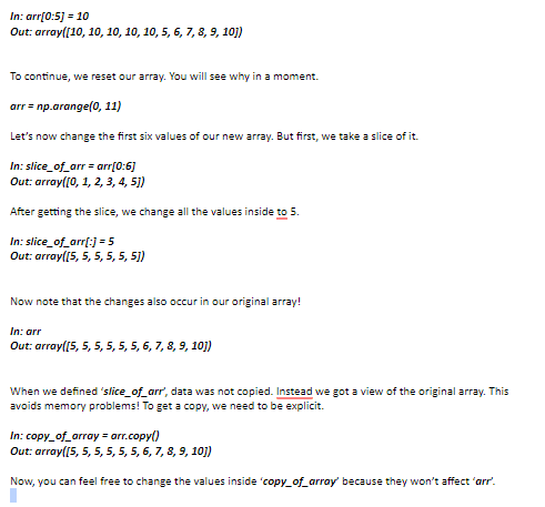
NumPy - Copies & Views
While executing the functions, some of them return a copy of the input array, while some return the view. When the contents are physically stored in another location, it is called Copy. If on the other hand, a different view of the same memory content is provided, we call it as View.
No Copy
Simple assignments do not make the copy of array object. Instead, it uses the same id() of the original array to access it. The id() returns a universal identifier of Python object, similar to the pointer in C.
Furthermore, any changes in either gets reflected in the other. For example, the changing shape of one will change the shape of the other too.
View or Shallow Copy
NumPy has ndarray.view() method which is a new array object that looks at the same data of the original array. Unlike the earlier case, change in dimensions of the new array doesn’t change dimensions of the original.
NumPy - Matrix Library
NumPy package contains a Matrix library numpy.matlib. This module has functions that return matrices instead of ndarray objects.
matlib.empty()
The matlib.empty() function returns a new matrix without initializing the entries. The function takes the following parameters.
numpy.matlib.empty(shape, dtype, order)
Where,
| Sr.No. | Parameter & Description |
| 1 | shapeint or tuple of int defining the shape of the new matrix |
| 2 | DtypeOptional. Data type of the output |
| 3 | orderC or F |
Example
import numpy.matlib
import numpy as np
print np.matlib.empty((2,2))
# filled with random data
It will produce the following output −
[[ 2.12199579e-314, 4.24399158e-314]
[ 4.24399158e-314, 2.12199579e-314]]
numpy.matlib.eye()
This function returns a matrix with 1 along the diagonal elements and the zeros elsewhere. The function takes the following parameters.
numpy.matlib.eye(n, M,k, dtype)
Where,
| Sr.No. | Parameter & Description |
| 1 | nThe number of rows in the resulting matrix |
| 2 | MThe number of columns, defaults to n |
| 3 | kIndex of diagonal |
| 4 | dtypeData type of the output |
Example
import numpy.matlib
import numpy as np
print np.matlib.eye(n = 3, M = 4, k = 0, dtype = float)
It will produce the following output −
[[ 1. 0. 0. 0.]
[ 0. 1. 0. 0.]
[ 0. 0. 1. 0.]]
NumPy - Matplotlib
Matplotlib is a plotting library for Python. It is used along with NumPy to provide an environment that is an effective open-source alternative for MatLab. It can also be used with graphics toolkits like PyQt and wxPython.
Matplotlib module was first written by John D. Hunter. Since 2012, Michael Droettboom is the principal developer. Currently, Matplotlib ver. 1.5.1 is the stable version available. The package is available in binary distribution as well as in the source code form on www.matplotlib.org.
Conventionally, the package is imported into the Python script by adding the following statement −
from matplotlib import pyplot as plt
Here pyplot() is the most important function in matplotlib library, which is used to plot 2D data. The following script plots the equation y = 2x + 5
Example:
import numpy as np
from matplotlib import pyplot as plt
x = np.arange(1,11)
y = 2 * x + 5
plt.title("Matplotlib demo")
plt.xlabel("x axis caption")
plt.ylabel("y axis caption")
plt.plot(x,y)
plt.show()
An ndarray object x is created from np.arange() function as the values on the x axis. The corresponding values on the y axis are stored in another ndarray object y. These values are plotted using plot() function of pyplot submodule of matplotlib package.
The graphical representation is displayed by show() function.
Instead of the linear graph, the values can be displayed discretely by adding a format string to the plot() function. Following formatting characters can be used.
NumPy - Using Matplotlib
NumPy has a numpy.histogram() function that is a graphical representation of the frequency distribution of data. Rectangles of equal horizontal size corresponding to class interval called bin and variable height corresponding to frequency.
numpy.histogram()
The numpy.histogram() function takes the input array and bins as two parameters. The successive elements in bin array act as the boundary of each bin.
import numpy as np
a = np.array([22,87,5,43,56,73,55,54,11,20,51,5,79,31,27])
np.histogram(a,bins = [0,20,40,60,80,100])
hist,bins = np.histogram(a,bins = [0,20,40,60,80,100])
print hist
print bins
It will produce the following output −
[3 4 5 2 1]
[0 20 40 60 80 100]
plt()
Matplotlib can convert this numeric representation of histogram into a graph. The plt() function of pyplot submodule takes the array containing the data and bin array as parameters and converts into a histogram.
from matplotlib import pyplot as plt
import numpy as np
a = np.array([22,87,5,43,56,73,55,54,11,20,51,5,79,31,27])
plt.hist(a, bins = [0,20,40,60,80,100])
plt.title("histogram")
plt.show()
It should produce the following output –
I/O with NumPy
The ndarray objects can be saved to and loaded from the disk files. The IO functions available are −
- load() and save() functions handle /numPy binary files (with npy extension)
- loadtxt() and savetxt() functions handle normal text files
NumPy introduces a simple file format for ndarray objects. This .npy file stores data, shape, dtype and other information required to reconstruct the ndarray in a disk file such that the array is correctly retrieved even if the file is on another machine with different architecture.
numpy.save()
The numpy.save() file stores the input array in a disk file with npy extension.
import numpy as np
a = np.array([1,2,3,4,5])
np.save('outfile',a)
To reconstruct array from outfile.npy, use load() function.
import numpy as np
b = np.load('outfile.npy')
print b
It will produce the following output −
array([1, 2, 3, 4, 5])
The save() and load() functions accept an additional Boolean parameter allow_pickles. A pickle in Python is used to serialize and de-serialize objects before saving to or reading from a disk file.
savetxt()
The storage and retrieval of array data in simple text file format is done with savetxt() and loadtxt() functions.
Example
import numpy as np
a = np.array([1,2,3,4,5])
np.savetxt('out.txt',a)
b = np.loadtxt('out.txt')
print b
It will produce the following output −
[ 1. 2. 3. 4. 5.]
We’d also recommend you to visit Great Learning Academy, where you will find a free NumPy course and 1000+ other courses. You will also receive a certificate after the completion of these courses. We hope that this Python NumPy Tutorial was beneficial and you are now better equipped.
NumPy Copy vs View
The difference between copy and view of an array in NumPy is that the view is merely a view of the original array whereas copy is a new array. The copy will not affect the original array and the chances are restricted to the new array created and many modifications made to the original array will not be reflected in the copy array too. But in view, the changes made to the view will be reflected in the original array and vice versa.
Let us understand with code snippets:
Example of Copy:
import numpy as np
arr1 = np.array([1, 2, 3, 4, 5])
y = arr1.copy()
arr1[0] = 36
print(arr1)
print(y)
Output :
[42 2 3 4 5]
[1 2 3 4 5]
Example of view:
Notice the output of the below code; the changes made to the original array are also reflected in the view.
import numpy as np
arr1 = np.array([1, 2, 3, 4, 5])
y= arr1.view()
arr1[0] = 36
print(arr1)
print(y)
Output:
[36 2 3 4 5]
[36 2 3 4 5]
NumPy Array Shape
The shape of an array is nothing but the number of elements in each dimension. To get the shape of an array, we can use a .shape attribute that returns a tuple indicating the number of elements.
import numpy as np
array1 = np.array([[2, 3, 4,5], [ 6, 7, 8,9]])
print(array1.shape)
Output: (2,4) NumPy Array Reshape
1-D to 2-D:
Array reshape is nothing but changing the shape of the array, through which one can add or remove a number of elements in each dimension. The following code will convert a 1-D array into 2-D array. The resulting will have 3 arrays having 4 elements
import numpy as np
array_1 = np.array([1, 2, 3, 4, 5, 6, 7, 8, 9, 10, 11, 12])
newarr1 = array_1.reshape(3, 4)
print(newarr1)
Output:
[[ 1 2 3 4]
[ 5 6 7 8]
[ 9 10 11 12]]
1-D to 3-D:
The outer dimension will contain two arrays that have three arrays with two elements each.
import numpy as np
array_1= np.array([1, 2, 3, 4, 5, 6, 7, 8, 9, 10, 11, 12])
newarr1 = array_1.reshape(2, 3, 2)
print(newarr1)
Output:
[[[ 1 2]
[ 3 4]
[ 5 6]]
[[ 7 8]
[ 9 10]
[11 12]]]
Flattening arrays:
Converting higher dimensions arrays into one-dimensional arrays is called flattening of arrays.
import numpy as np
arr1= np.array([[4,5,6], [7, 8, 9]])
newarr1 = arr1.reshape(-1)
print(newarr1)
Output :
[1 2 3 4 5 6]
NumPy Array Iterating
Iteration through the arrays is possible using for loop.
Example 1:
import numpy as np
arr1 = np.array([1, 2, 3])
for i in arr1:
print(i)
Output: 1
2
3
Example 2:
import numpy as np
arr = np.array([[4, 5, 6], [1, 2, 3]])
for x in arr:
print(x)
Output: [4, 5, 6]
[1, 2, 3]
Example3:
import numpy as np
array1 = np.array([[1, 2, 3], [4, 5, 6]])
for x in array1:
for y in x:
print(y)
NumPy Array Join
Joining is an operation of combining one or two arrays into a single array. In Numpy, the arrays are joined by axes. The concatenate() function is used for this operation, it takes a sequence of arrays that are to be joined, and if the axis is not specified, it will be taken as 0.
import numpy as np
arr1 = np.array([1, 2, 3])
arr2 = np.array([4, 5, 6])
finalarr = np.concatenate((arr1, arr2))
print(finalarr)
Output: [1 2 3 4 5 6]
The following code joins the specified arrays along the rows
import numpy as np
arr1 = np.array([[1, 2], [3, 4]])
arr2 = np.array([[5, 6], [7, 8]])
finalarr = np.concatenate((arr1, arr2), axis=1)
print(finalarr)
Output:
[[1 2 5 6]
[3 4 7 8]]
NumPy Array Split
As we know, split does the opposite of join operation. Split breaks a single array as specified. The function array_split() is used for this operation and one has to pass the number of splits along with the array.
import numpy as np
arr1 = np.array([7, 8, 3, 4, 1, 2])
finalarr = np.array_split(arr1, 3)
print(finalarr)
Output: [array([7, 8]), array([3, 4]), array([1, 2])]
Look at an exceptional case where the no of elements is less than required and observe the output
Example :
import numpy as np
array_1 = np.array([4, 5, 6,1,2,3])
finalarr = np.array_split(array_1, 4)
print(finalarr)
Output : [array([4, 5]), array([6, 1]), array([2]), array([3])]
Split into Arrays
The array_split() will return an array containing an array as a split, we can access the elements just as we do in a normal array.
import numpy as np
array1 = np.array([4, 5, 6,7,8,9])
finalarr = np.array_split(array1, 3)
print(finalarr[0])

print(finalarr[1])
Output :
[4 5]
[6 7]
Splitting of 2-D arrays is also similar, send the 2-d array in the array_split()
import numpy as np
arr1 = np.array([[1, 2], [3, 4], [5, 6], [7, 8], [9, 10], [11, 12]])
finalarr = np.array_split(arr1, 3)
print(finalarr)
Output:
[array([[1, 2],
[3, 4]]), array([[5, 6],
[7, 8]]), array([[ 9, 10],
[11, 12]])]
NumPy Array Search
The where() method is used to search an array. It returns the index of the value specified in the where method.
The below code will return a tuple indicating that element 4 is at 3,5 and 6
import numpy as np
arr1 = np.array([1, 2, 3, 4, 5, 4, 4])
y = np.where(arr1 == 4)
print(y)
Output : (array([3, 5, 6]),)
Built-In Methods
Numpy allows us to use many built-in methods for generating arrays. Let’s examine the most used from those, as well as their purpose:
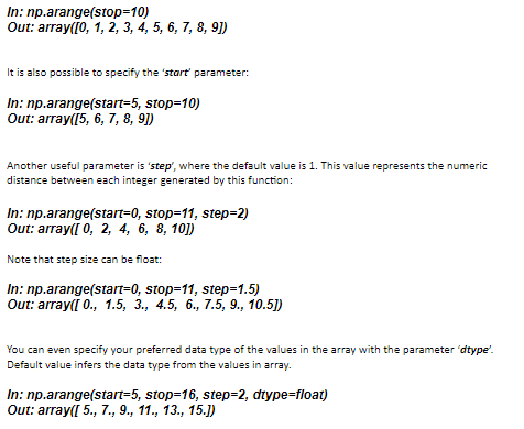
np.arange() - array of arranged values from low to high value
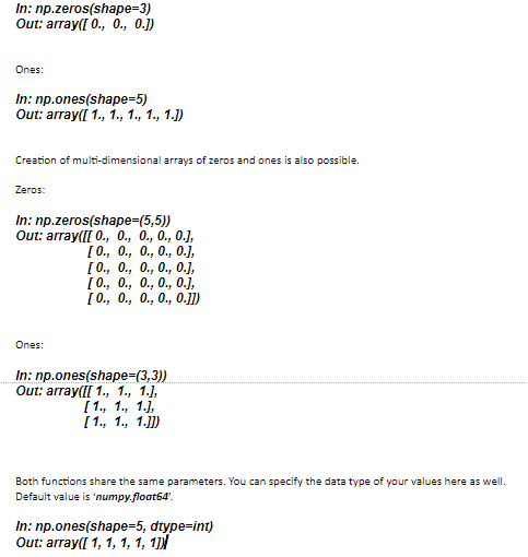
np.zeros() - array of zeros with specified shape
np.ones() - similarly to zeros, array of ones with specified shape
np.linspace() - array of linearly spaced numbers, with specified size
np.eye() - two dimensional array with ones on the diagonal, zeros elsewhere
Arange
Numpy’s arange function will return evenly spaced values within a given interval. Works similarly to Python’s range() function. The only required parameter is ‘stop’, while all the other parameters are optional:
Zeros and ones
Numpy provides functions that are able to create arrays of 1’s and 0’s. The required parameter for these functions is ‘shape’.
Create array filled with zero values:
Linspace
Numpy’s linspace function will return evenly spaced numbers over a specified interval. Required parameters for this functions are ‘start’ and ‘stop’.
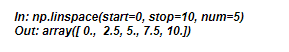
The parameter ‘num’ specifies the number of samples to generate, and the default value is 50. The value defined in the parameter ‘num’ must be non-negative. You are able to change the data type of your values using ‘dtype’ as parameter.
Eye
Numpy’s eye function will return Identity Matrix. The identity matrix is a square matrix that has 1’s along the main diagonal and 0’s for all other entries. This matrix is often written simply as ‘I’, and is special in that it acts like 1 in matrix multiplication. Required parameter for this function is ‘N’, number of rows in the output.
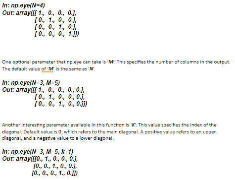
Specification of a data type of the matrix’s values using ‘dtype’ is also possible.
Random
Numpy allows you to use various functions to produce arrays with random values. To access these functions, first we have to access the ‘random’ function itself. This is done using ‘np.random’, after which we specify which function we need. Here is a list of the most used random functions and their purpose:
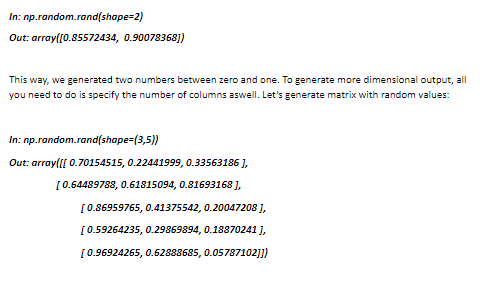
np.random.rand() – produce random values in the given shape from 0 to 1
np.random.randn() - produce random values with a ‘standard normal’ distribution, from -1 to 1
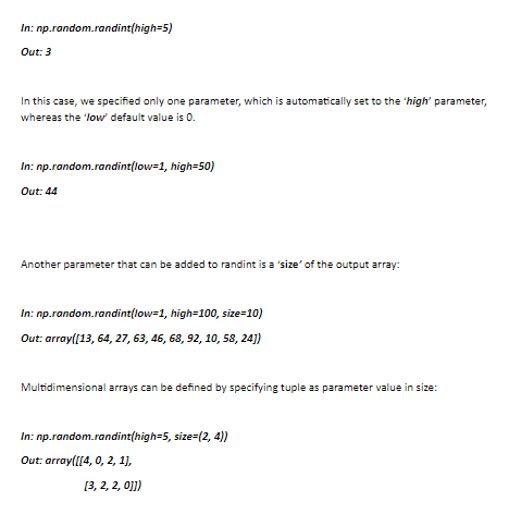
np.random.randint() - produce random numbers from low to high, specified as parameter
Rand
The rand function uses only one parameter which is the ‘shape’ of the output. You need to specify the output format you need, whether it is one or two dimensional array. If there is no argument passed to the function, it returns a single value. Otherwise, it produces number of numbers as specified. For example:
Randn
The randn function is similar to the rand function, except it produces a number with standard normal distribution. What this means, is that it generates number with distribution of 1 and mean of 0, i.e. value from -1 to +1 by default:
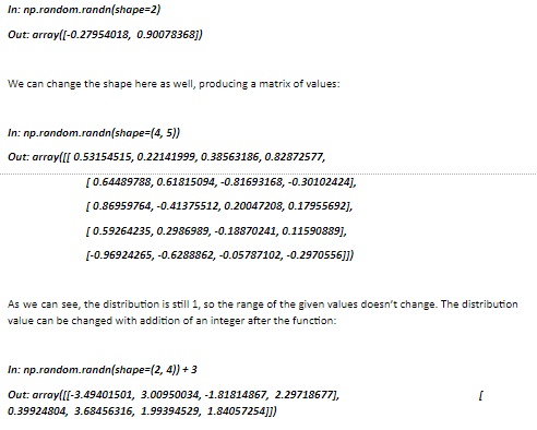
The distribution is now equal to 4, so the given floats vary between minus and plus 4. Other mathematical operations such as multiplication, division, subtraction are possible in order to modify the distribution, depending on the needs.
Randint
Randint is used to generate whole random numbers, ranging between low(inclusive) and high(exclusive) value. Specifying a parameter like ‘(1, 100)’ will create random values from 1 to 99.
Array Attributes and Methods
Now we will continue with more attributes and methods that can be used on arrays. In this lecture we will talk about:
Reshape – changes the shape of an array into the desired shape
Shape – returns the shape of the given array as parameter
Dtype – returns the data type of the values in the array
These methods will improve your ‘trial-and-error’, meaning, once you find yourself in a situation where you encounter an error, applying methods like this may help you locate the error faster, thus it will save you a lot of time in the future. Let’s dive straight in.
Reshape
This method allows you to transform one dimensional array to more dimensional, or the other way around. Reshape will not affect your data values. Let’s check out this code:
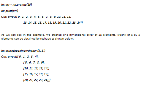
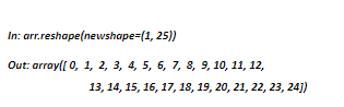
The array named ‘arr’ is now reshaped into a 5 by 5 matrix and by this, we specify the number of rows and the number of columns. Key thing to notice is that the array still has all 25 elements. Reshaping it into a 4 by 5 matrix(4 rows, 5 columns), would’ve produced an error since the reshape size is not the same size as the array’s. It would’ve been possible if the array had only 20 elements. To reverse the process and return the array into it’s original shape, we could do this:
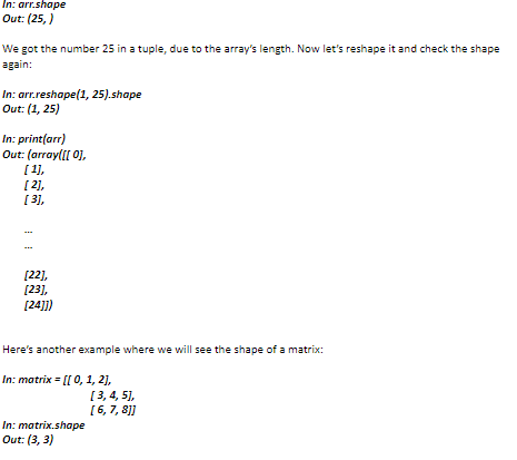
Shape
The ‘shape’ method will return you a tuple consisting of the array’s dimensions. Let’s check out the shape of the previously used array:
Dtype
This function allows you to check the data type of the array’s values.
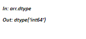
There can be more the one data type present in an array, so make sure to check Numpy’s documentation on ‘dtypes’ for more.
Numpy Indexing and Selection
In this lecture, we will discuss how to select element or groups of elements from an array and change them. Here is a list of what we will cover in this lecture:
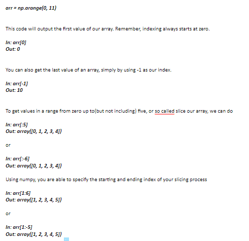
Indexing – pick one or more elements from an array
Broadcasting – changing values within an index range
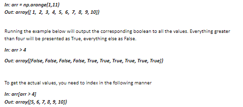
Bracket Indexing and Selection
The simplest way to pick one or more elements of an array looks very similar to Python lists. We will be using the following array as an example
Broadcasting
Numpy arrays differ from a normal Python list because of their ability to broadcast. Below is an example of setting a value within index range (Broadcasting).
Indexing 2D Array/Matrix
The main idea behind this lecture is to help you get comfortable with indexing in more than 1 dimensions. Below is a list of what we will cover.
Indexing a 2D array – Indexing matrices differs from vectors
Fancy indexing – Selecting entire rows or columns out of order
Selection – Selection based off of comparison operators
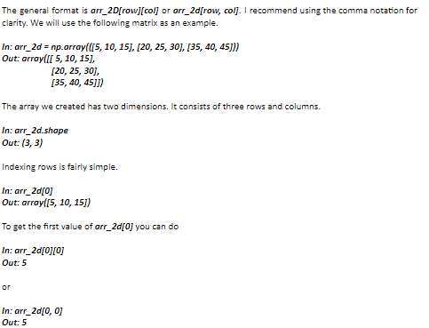
They both work. Throughout this lecture we will be using the second notation.
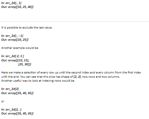
Now, how do you index a column? I will show you an example of selecting the second column with all the values inside.
You can see that both examples provide the same output. In these kinds of cases, using the first example is recommended for the sake of simplicity.
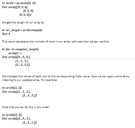
Fancy Indexing
Fancy indexing allows you to select entire rows or columns out of order. To show this, let's quickly build out a numpy array of zeros.
Selection
Let's briefly go over how to use brackets for selection based off of comparison operators. But first we need to create an array we will use as an example.
Numpy Operations
We can perform different types of operations on NumPy arrays. What this means is we can sum, subtract, multiply or divide the values inside our array, even do things like taking the square root. Below is a list of what we will cover in this lecture.
Arithmetic Operations – sum, subtract, multiply, divide on arrays
Universal Array Functions – Mathematical operations provided by NumPy
Arithmetic
While performing arithmetic operations between two arrays it is important that they have the same dimensions. We will use the following array as an example
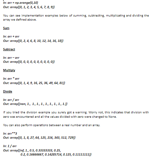
If you run the last example you will again get a warning for dividing with zero. Note that this time instead of None, we get a value of infinity.
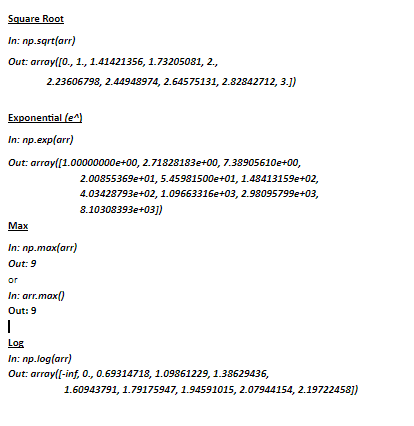
Universal Array Functions
Numpy comes with many universal array functions, which are essentially just mathematical operations you can use to perform the operation across the array. Let's show some common ones.
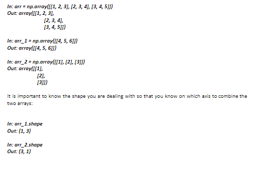
When dealing with messy data you will often need to stick multiple arrays together. In this lecture we will cover how this is done using numpy. Another list of what we will cover:
Append, Concatenate and Stack
Append – append one array to another
Concatenate – Concatenate two arrays
Stack – Stack one array to another horizontally or vertically
These functions don’t work in-place, meaning you need to put your combined arrays to a new variable. Throughout this lecture we will be using the following arrays as an example:
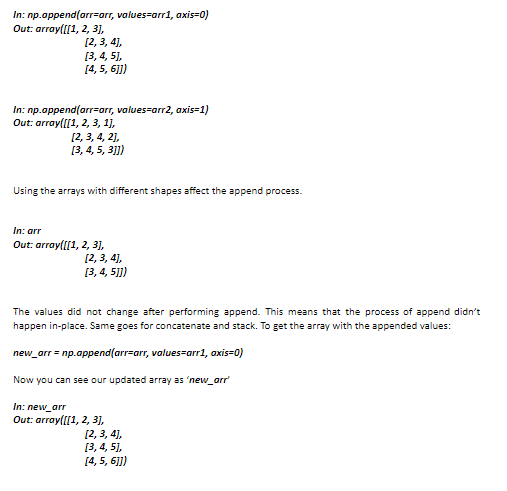
Append
To append using numpy we use np.append() function which requires three parameters, ‘arr’, ‘values’ and ‘axis’ on which to append.
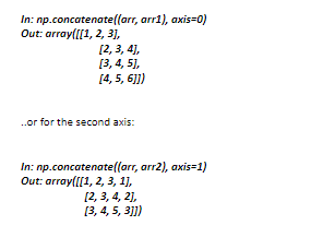
Concatenate
Concatenate works similarly to append, but instead of ‘arr’ and ‘values’ as parameters it takes a tuple of two arrays. Let’s show you few examples.
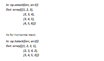
Stack
There are two ways of stacking arrays together, horizontally and vertically. Example for vertical stack:
Watch the following video to understand how NumPy Scikit works in Machine Learning.
Frequently Asked Questions on NumPy in Python
1. What is NumPy and why is it used in Python?
Numpy- Also known as numerical Python, is a library used for working with arrays. It is also a general-purpose array-processing package that provides comprehensive mathematical functions, linear algebra routines, Fourier transforms, and more.
NumPy aims to provide less memory to store the data compared to python list and also helps in creating n-dimensional arrays. This is the reason why NumPy is used in Python.
2. How do you define a NumPy in Python?
NumPy in python is defined as a fundamental package for scientific computing that helps in facilitating advanced mathematical and other types of operations on large numbers of data.
3. Where is NumPy used?
NumPy is a python library mainly used for working with arrays and to perform a wide variety of mathematical operations on arrays.NumPy guarantees efficient calculations with arrays and matrices on high-level mathematical functions that operate on these arrays and matrices.
4. Should I use NumPy or pandas?
Go through the below points and decide whether to use NumPy or Pandas, here we go:
- NumPy and Pandas are the most used libraries in Data Science, ML and AI.
- NumPy and Pandas are used to save n number of lines of Codes.
- NumPy and Pandas are open source libraries.
- NumPy is used for fast scientific computing and Pandas is used for data manipulation, analysis and cleaning.
5. What is the difference between NumPy and pandas?
| NumPy | Pandas |
| Numpy creates an n-dimensional array object. | Pandas create DataFrame and Series. |
| Numpy array contains data of same data types | Pandas is well suited for tabular data |
| Numpy requires less memory | Pandas required more memory compared to NumPy |
| NumPy supports multidimensional arrays. | Pandas support 2 dimensional arrays |
6. What is a NumPy array?
Numpy array is formed by all the computations performed by the NumPy library. This is a powerful N-dimensional array object with a central data structure and is a collection of elements that have the same data types.
7. What is NumPy written in?
NumPy is a Python library that is partially written in Python and most of the parts are written in C or C++. And it also supports extensions in other languages, commonly C++ and Fortran.
8. Is NumPy easy to learn?
NumPy is an open-source Python library that is mainly used for data manipulation and processing in the form of arrays.NumPy is easy to learn as it works fast, works well with other libraries, has lots of built-in functions, and lets you do matrix operations.
NumPy is a fundamental Python library that gives you access to powerful mathematical functions. If you're looking to dive deep into scientific computing and data analysis, then NumPy is definitely the way to go.
On the other hand, pandas is a data analysis library that makes it easy to work with tabular data. If your focus is on business intelligence and data wrangling, then pandas are the library for you.
In the end, it's up to you which one you want to learn first. Just be sure to focus on one at a time, and you'll be mastering NumPy in no time!
Embarking on a journey towards a career in data science opens up a world of limitless possibilities. Whether you’re an aspiring data scientist or someone intrigued by the power of data, understanding the key factors that contribute to success in this field is crucial. The below path will guide you to become a proficient data scientist.