
In this tutorial, we are going to start from scratch and see how to use SciPy, scipy in python and introduce you to some of its most important features. Also, we are going to go through the different modules or sub-packages present in the SciPy package and see how they are used.
In this course, you will learn the fundamentals of Python: from basic syntax to mastering data structures, loops, and functions. You will also explore OOP concepts and objects to build robust programs.
What is SciPy?
SciPy is a free and open-source Python library used for scientific computing and technical computing. It is a collection of mathematical algorithms and convenience functions built on the NumPy extension of Python. It adds significant power to the interactive Python session by providing the user with high-level commands and classes for manipulating and visualizing data. As mentioned earlier, SciPy builds on NumPy and therefore if you import SciPy, there is no need to import NumPy.
Installing SciPy
Before learning more about the core functionality of SciPy, it should be installed in the system.
Install on Windows and Linux
Here are a few methods that can be used to install SciPy on Windows or Linux.
Install SciPy using pip
We can install the SciPy library by using the pip command. Pip is basically a recursive acronym which stands for ‘Pip Installs Packages’. It is a standard package manager which can be installed in most of the operating systems. To install, run the following command in the terminal:
pip install scipy
Note: Use pip to install SciPy in Linux.
Install SciPy using Anaconda
We can also install SciPy packages by using Anaconda. First, we need to download the Anaconda navigator and then open the anaconda prompt type the following command:
conda install -c anaconda scipy
Install on Mac
The mac doesn't have the preinstall package manager, but you can install various popular package managers. Run the following commands in the terminal it will download the SciPy as well as matplotlib, pandas, NumPy.
sudo port install py35-numpy py35-scipy py35-matplotlib py35-ipython +notebook py35-pandas py35-sympy py35-nose
Also, you can use Homebrew to install these packages. But keep in mind that it has incomplete coverage of the SciPy ecosystem:
brew install numpy scipy ipython jupyter
Sub packages in SciPy
Many dedicated software tools are necessary for Python scientific computing, and SciPy is one such tool or library offering many Python modules that we can work with in order to perform complex operations.
The following table shows some of the modules or sub-packages that can be used for computing:
| Sr. | Sub-Package | Description |
| 1. | scipy.cluster | Cluster algorithms are used to vector quantization/ Kmeans. |
| 2. | scipy.constants | It represents physical and mathematical constants. |
| 3. | scipy.fftpack | It is used for Fourier transform. |
| 4. | scipy.integrate | Integration routines |
| 5. | scipy.interpolation | Interpolation |
| 6. | scipy.linalg | It is used for linear algebra routine. |
| 7. | scipy.io | It is used for data input and output. |
| 8. | scipy.ndimage | It is used for the n-dimension image. |
| 9. | scipy.odr | Orthogonal distance regression. |
| 10. | scipy.optimize | It is used for optimization. |
| 11. | scipy.signal | It is used in signal processing. |
| 12. | scipy.sparse | Sparse matrices and associated routines. |
| 13. | scipy.spatial | Spatial data structures and algorithms. |
| 14. | scipy.special | Special Function. |
| 15. | scipy.stats | Statistics. |
| 16. | scipy.weaves | It is a tool for writing. |
SciPy Cluster
Clustering is the task of dividing the population or data points into a number of groups such that data points in the same groups are more similar to other data points in the same group and dissimilar to the data points in other groups. Each group which is formed from clustering is known as a cluster. There are two types of the cluster, which are:
- Central
- Hierarchy
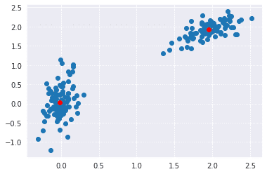
Here we will see how to implement the K-means clustering algorithm which is one of the popular clustering algorithms. The k-means algorithm adjusts the classification of the observations into clusters and updates the cluster centroids until the position of the centroids is stable over successive iterations.
In the below implementation, we have used NumPy to generate two sets of random points. After joining both these sets, we whiten the data. Whitening normalizes the data and is an essential step before using k-means clustering. Finally, we use the kmeans functions and pass it the data and number of clustered we want.
import numpy as np
from scipy.cluster.vq import  kmeans, whiten
import matplotlib.pyplot as plt
import seaborn as sns
sns.set_style("darkgrid")
# Create 50 datapoints in two clusters a and b
pts = 100
a = np.random.multivariate_normal([0, 0],
                                  [[4, 1], [1, 4]],
                                  size=pts)
b = np.random.multivariate_normal([30, 10],
                                  [[10, 2], [2, 1]],
                                  size=pts)
features = np.concatenate((a, b))
# Whiten data
whitened = whiten(features)
# Find 2 clusters in the data
codebook, distortion = kmeans(whitened, 2)
# Plot whitened data and cluster centers in red
plt.scatter(whitened[:, 0], whitened[:, 1])
plt.scatter(codebook[:, 0], codebook[:, 1], c='r')
plt.show()
Output:
SciPy constants
There are a variety of constants that are included in the scipy.constant sub-package.These constants are used in the general scientific area. Let us see how these constant variables are imported and used.
#Import golden constant from the scipy
import scipy
print("sciPy -golden ratio  Value = %.18f"%scipy.constants.golden)
Output:
sciPy -golden ratio  Value = 1.618033988749894903
As you can see, we imported and printed the golden ratio constant using SciPy.The scipy.constant also provides the find() function, which returns a list of physical_constant keys containing a given string.
Consider the following example:
from scipy.constants import find
find('boltzmann')
 Output:
['Boltzmann constant',
 'Boltzmann constant in Hz/K',
 'Boltzmann constant in eV/K',
 'Boltzmann constant in inverse meter per kelvin',
 'Stefan-Boltzmann constant']
Here is how you can get the value of the required constant:
scipy.constants.physical_constants['Boltzmann constant in Hz/K']
Now let us see the list of constants that are included in this subpackage. The scipy.constant provides the following list of mathematical constants.
| Sr. No. | Constants | Description |
| 1. | pi | pi |
| 2. | golden | Golden ratio |
The scipy.constant.physical_sconstants provides the following list of physical constants.
| Sr. No. | Physical Constants | Description |
| 1. | c | Speed of light in vacuum |
| 2. | speed_of_light | Speed of light in vacuum |
| 3. | G | Standard acceleration of gravity |
| 4. | G | Newton Constant of gravitation |
| 5. | E | Elementary charge |
| 6. | R | Molar gas constant |
| 7. | Alpha | Fine-structure constant |
| 8. | N_A | Avogadro constant |
| 9. | K | Boltzmann constant |
| 10 | Sigma | Stefan-Boltzmann constant σ |
| 11. | m_e | Electron mass |
| 12. | m_p | Proton mass |
| 13. | m_n | Neutron Mass |
| 14. | H | Plank Constant |
| 15. | Plank constant | Plank constant h |
Here is a complete list of constants that are included in the constant subpackage.
SciPy FFTpack
The FFT stands for Fast Fourier Transformation which is an algorithm for computing DFT. DFT is a mathematical technique which is used in converting spatial data into frequency data.
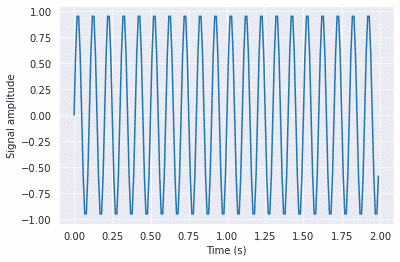
SciPy provides the fftpack module, which is used to calculate Fourier transformation. In the example below, we will plot a simple periodic function of sin and see how the scipy.fft function will transform it.
from matplotlib import pyplot as plt
import numpy as np
import seaborn as sns
sns.set_style("darkgrid")
#Frequency in terms of Hertz
fre  = 10
#Sample rate
fre_samp = 100
t = np.linspace(0, 2, 2 * fre_samp, endpoint = False )
a = np.sin(fre  * 2 * np.pi * t)
plt.plot(t, a)
plt.xlabel('Time (s)')
plt.ylabel('Signal amplitude')
plt.show()
Output:
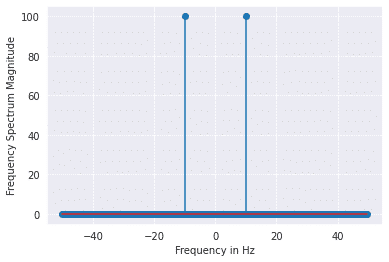
from scipy import fftpack
A = fftpack.fft(a)
frequency = fftpack.fftfreq(len(a)) * fre_samp
plt.stem(frequency, np.abs(A),use_line_collection=True)
plt.xlabel('Frequency in Hz')
plt.ylabel('Frequency Spectrum Magnitude')
plt.show()
Output:
This subpackage also provides us functions such as fftfreq() which will generate the sampling frequencies. Also fftpack.dct() function allows us to calculate the Discrete Cosine Transform (DCT).SciPy also provides the corresponding IDCT with the function idct().
SciPy integrate
The integrate sub package of the Scipy package contains a lot of functions that allow us to calculate the integral of some complex functions. If you use the help function, you will find all the different types of integrals you can calculate. Here is how:
help(integrate)
 Methods for Integrating Functions given function object.

   quad          -- General purpose integration.
   dblquad       -- General purpose double integration.
   tplquad       -- General purpose triple integration.
   fixed_quad    -- Integrate func(x) using Gaussian quadrature of order n.
   quadrature    -- Integrate with given tolerance using Gaussian quadrature.
   romberg       -- Integrate func using Romberg integration.

 Methods for Integrating Functions given fixed samples.

   trapz         -- Use trapezoidal rule to compute integral from samples.
   cumtrapz      -- Use trapezoidal rule to cumulatively compute integral.
   simps         -- Use Simpson's rule to compute integral from samples.
   romb          -- Use Romberg Integration to compute integral from
                    (2**k + 1) evenly-spaced samples.

   See the special module's orthogonal polynomials (special) for Gaussian
      quadrature roots and weights for other weighting factors and regions.

 Interface to numerical integrators of ODE systems.

   odeint        -- General integration of ordinary differential equations.
   ode           -- Integrate ODE using VODE and ZVODE routines.
So as you can see we have a wide variety of functions, now let us use a few of them here:
Single Integrals:
We use the quad function to calculate the single integral of a function. Numerical integrate is sometimes called quadrature and hence the name quad. The function has three parameters:
scipy.integrate.quad(f,a,b)
 f - Function to be integrated.
 a-lower limit.
 b- upper limit.
Here is an example where we use this function:
First, let us define a function using lambda function as shown below:
from numpy import exp
f= lambda x:exp(-x**2)
Remember, quad() function expects us to pass a function, thus we used lambda to form a function rather than using an expression.Now to calculate the integral:
import scipy
i = scipy.integrate.quad(f, 0, 1)
print(i)
 Output:
(0.7468241328124271, 8.291413475940725e-15)
The first value is the tuple is the integral value with upper limit one and lower limit zero.Also, the second value is an estimate of the absolute error in the value of an integer.
Multiple Integrals
There are various functions such as dblquad(), tplquad(), and nquad() that enable us to calculate multiple integrals.the dblquad() function and tplquad() functions calculate the double and triple integrals respectively,whereas nquad performs n-fold multiple integration.
Below we will use scipy.integrate.dblquad(func,a,b,gfun,hfun) to solve double integrals. The first argument func is the name of the function to be integrated and a and b are the lower and upper limit of the x variable. While gfun and hfun are names of the functions that define the lower and upper limit of the y variable.It is important to note that that limits of inner integrals must be passed functions as in the following example:
import scipy.integrate
from numpy import exp
from math import sqrt
f = lambda x, y : 2*x*y
g = lambda x : 0
h = lambda y : 4*y**2
i = scipy.integrate.dblquad(f, 0, 0.5, g, h)
print(i)
 Output:
(0.04166666666666667, 5.491107323698757e-15)
SciPy Interpolation
Interpolation is the process of estimating unknown values that fall between known values.SciPy provides us with a sub-package scipy.interpolation which makes this task easy for us. Using this package, we can perform 1-D or univariate interpolation and Multivariate interpolation. Multivariate interpolation (spatial interpolation ) is a kind interpolation on functions that consist of more than one variables.
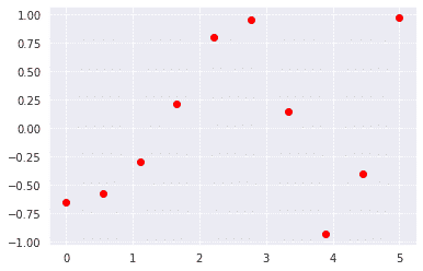
Here is an example of 1-D interpolation where there is only variable i.e. ‘x’:
First, we will define some points and plot them
import numpy as np
from scipy import interpolate
import matplotlib.pyplot as plt
x = np.linspace(0, 5, 10)
y = np.cos(x**2/3+4)
plt.scatter(x,y,c='r')
plt.show()
Output:
scipy.interpolation provides interp1d class which is a useful method to create a function based on fixed data points. We will create two such functions that use different techniques of interpolation. The difference will be clear to you when you see the plotted graph of both of these functions.
from scipy.interpolate import interp1d
import matplotlib.pyplot as plt
fun1 = interp1d(x, y,kind = 'linear')
fun2 = interp1d(x, y, kind = 'cubic')
#we define a new set of input
xnew = np.linspace(0, 4,30)
plt.plot(x, y, 'o', xnew, fun1(xnew), '-', xnew, fun2(xnew), '--')
plt.legend(['data', 'linear', 'cubic','nearest'], loc = 'best')
plt.show()
Output:
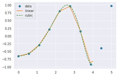
In the above program, we have created two functions fun1 and fun2. The variable x contains the sample points, and variable y contains the corresponding values. The third variable kind represents the types of interpolation techniques. There are various methods of interpolation. These methods are the following:
- Linear
- Nearest
- Zero
- S-linear
- Quadratic
- Cubic
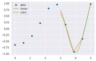
Now what happens when we change the input values
from scipy.interpolate import interp1d
import matplotlib.pyplot as plt
fun1 = interp1d(x, y,kind = 'linear')
fun2 = interp1d(x, y, kind = 'cubic')
xnew = np.linspace(3, 5,30)
plt.plot(x, y, 'o', xnew, fun1(xnew), '-', xnew, fun2(xnew), '--')
plt.legend(['data', 'linear', 'cubic','nearest'], loc = 'best')
plt.show()
Output:
SciPy linalg
SciPy has very fast linear algebra capabilities as it is built using the optimized ATLAS (Automatically Tuned Linear Algebra Software), LAPACK(Linear Algebra Package) and BLAS(Basic Linear Algebra Subprograms) libraries. All of these linear algebra routines can operate on an object that can be converted into a two-dimensional array and also returns the output as a two-dimensional array.
You might wonder that numpy.linalg also provides us with functions that help to solve algebraic equations, so should we use numpy.linalg or scipy.linalg? The scipy.linalg contains all the functions that are in numpy.linalg, in addition it also has some other advanced functions that are not in numpy.linalg. Another advantage of using scipy.linalg over numpy.linalg is that it is always compiled with BLAS/LAPACK support, while for NumPy this is optional, so it's faster as mentioned before.
Solve Linear Equations
We can use scipy.linalg.solve() to solve a linear equation, all we need to know is how to represent our equations in terms of vectors. Here is an example:
import numpy as np
from scipy import linalg
# We are trying to solve a linear algebra system which can be given as
#         x + 2y - 3z = -3
#         2x - 5y + 4z = 13
#         5x + 4y - z = 5
#We will find values of x,y and z for which all these equations are zero
#Also finally we will check if the values are right by substituting them
#in the equations
# Creating input array
a = np.array([[1, 2, -3], [2, -5, 4], [5, 4, -1]])
# Solution Array
b = np.array([[-3], [13], [5]])
# Solve the linear algebra
x = linalg.solve(a, b)
# Print results
print(x)
# Checking Results
print("n Checking results,must be zeros")
print(a.dot(x) - b)
 Output:
[[ 2.]
 [-1.]
 [ 1.]]

 Checking results, Vectors must be zeros
[[0.]
 [0.]
 [0.]]
As we can see, we got three values i.e 2,-1 and 1.So for x=2,y=-1 and z=1 the above three equations are zero as shown above.
Finding a determinant of a square matrix
The determinant is a scalar value that can be computed from the elements of a square matrix and encodes certain properties of the linear transformation described by the matrix. The determinant of a matrix A is denoted det, det A, or |A|. In SciPy, this is computed using the det() function. It takes a matrix as input and returns a scalar value.
#importing the scipy and numpy packages
from scipy import linalg
import numpy as np

#Declaring the numpy array
A = np.array([[1,2,9],[3,4,8],[7,8,4]])
#Passing the values to the det function
x = linalg.det(A)

#printing the result
print('Determinant of n{} n is {}'.format(A,x))
Output:
Determinant of
[[1 2 9]
 [3 4 8]
 [7 8 4]]
 is 3.999999999999986
Eigenvalues and Eigenvectors
For a square matrix(A) we can find the eigenvalues (λ) and the corresponding eigenvectors (v) of by considering the following relation
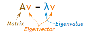
We can use scipy.linalg.eig to computes the eigenvalues and the eigenvectors for a particular matrix as shown below:
#importing the scipy and numpy packages
from scipy import linalg
import numpy as np

#Declaring the numpy array
A = np.array([[2,1,-2],[1,0,0],[0,1,0]])

#Passing the values to the eig function
values, vectors = linalg.eig(A)

#printing the result for eigenvalues
print(values)

#printing the result for eigenvectors
print(vectors)
 Output:
[-1.+0.j  2.+0.j  1.+0.j]
[[-0.57735027 -0.87287156  0.57735027]
 [ 0.57735027 -0.43643578  0.57735027]
 [-0.57735027 -0.21821789  0.57735027]]
SciPy IO (Input & Output)
The functions provided by the scipy.io package enables us to work around with different formats of files such as:
- Matlab
- IDL
- Matrix Market
- Wave
- Arff
- Netcdf, etc.
The functions such as loadmat(), savemat() and whosmat() can load a MATLAB file, save a MATLAB file and list variables in a MATLAB file respectively. Here is an example:
First, save a MatLab file as test.mat which contains a structure as shown below:
my_struct = struct('lon', 78, 'lat', 56)
Now we can use loadmat() function to import this file into a python script as shown below:
from scipy.io import loadmat
x = loadmat('test.mat')
#save the individual elements as python object
lon = x['lon']
lat = x['lat']
# one-liner to read a single variable
lon = loadmat('test.mat')['lon']
SciPy Ndimage
The SciPy provides the ndimage (n-dimensional image) package, that contains the number of general image processing and analysis functions. Some of the most common tasks in image processing are as follows:
- Basic manipulations − Cropping, flipping, rotating, etc.
- Image filtering − Denoising, sharpening, etc.
- Image segmentation − Labeling pixels corresponding to different objects
- Classification
- Feature extraction
- Registration
Here are some examples in which we will apply some of these image processing techniques on the images:
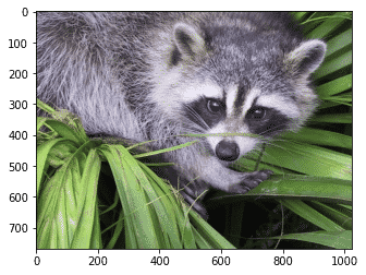
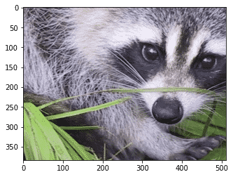
First, let us import an image that is already included in the SciPy package:
import scipy.misc
import matplotlib.pyplot as plt
face = scipy.misc.face()#returns an image of raccoon
#display image using matplotlib
plt.imshow(face)
plt.show()
Output:
Crop image
import scipy.misc
import matplotlib.pyplot as plt
face = scipy.misc.face()#returns an image of raccoon
lx,ly,channels= face.shape
# Cropping
crop_face = face[int(lx/4):int(-lx/4), int(ly/4):int(-ly/4)]
plt.imshow(crop_face)
plt.show()
Output:
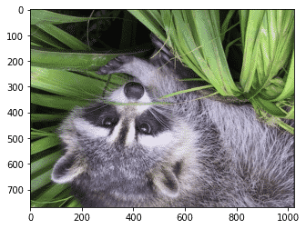
Rotate Image
from scipy import misc,ndimage
import matplotlib.pyplot as plt
face = misc.face()
rotate_face = ndimage.rotate(face, 180)
plt.imshow(rotate_face)
plt.show()
Output:
Blurring or Smoothing Images
Here we will blur the original images using the Gaussian filter and see how to control the level of smoothness using the sigma parameter.
from scipy import ndimage,misc
import matplotlib.pyplot as plt

face = scipy.misc.face(gray=True)
blurred_face = ndimage.gaussian_filter(face, sigma=3)
very_blurred = ndimage.gaussian_filter(face, sigma=5)

plt.figure(figsize=(9, 3))
plt.subplot(131)
plt.imshow(face, cmap=plt.cm.gray)
plt.axis('off')
plt.subplot(132)
plt.imshow(very_blurred, cmap=plt.cm.gray)
plt.axis('off')
plt.subplot(133)
plt.imshow(blurred_face, cmap=plt.cm.gray)
plt.axis('off')


plt.subplots_adjust(wspace=0, hspace=0., top=0.99, bottom=0.01,
                    left=0.01, right=0.99)

plt.show()
Output:

The first image is the original image followed by the blurred images with different sigma values.
Sharpening images
Here we will blur the image using the Gaussian method mentioned above and then sharpen the image by adding intensity to each pixel of the blurred image.
import scipy
from scipy import ndimage
import matplotlib.pyplot as plt

f = scipy.misc.face(gray=True).astype(float)
blurred_f = ndimage.gaussian_filter(f, 3)

filter_blurred_f = ndimage.gaussian_filter(blurred_f, 1)

alpha = 30
sharpened = blurred_f + alpha * (blurred_f - filter_blurred_f)

plt.figure(figsize=(12, 4))

plt.subplot(131)
plt.imshow(f, cmap=plt.cm.gray)
plt.axis('off')
plt.subplot(132)
plt.imshow(blurred_f, cmap=plt.cm.gray)
plt.axis('off')
plt.subplot(133)
plt.imshow(sharpened, cmap=plt.cm.gray)
plt.axis('off')

plt.tight_layout()
plt.show()
Output:

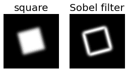
Edge detection
Edge detection includes a variety of mathematical methods that aim at identifying points in a digital image at which the image brightness changes sharply or, more formally, has discontinuities. The points at which image brightness changes sharply are typically organized into a set of curved line segments termed edges.
Here is an example where we make a square figure and then find its edges:
mport numpy as np
from scipy import ndimage
import matplotlib.pyplot as plt

im = np.zeros((256, 256))
im[64:-64, 64:-64] = 1

im = ndimage.rotate(im, 15, mode='constant')
im = ndimage.gaussian_filter(im, 8)

sx = ndimage.sobel(im, axis=0, mode='constant')
sy = ndimage.sobel(im, axis=1, mode='constant')
sob = np.hypot(sx, sy)

plt.figure(figsize=(9,5))
plt.subplot(141)
plt.imshow(im)
plt.axis('off')
plt.title('square', fontsize=20)
plt.subplot(142)
plt.imshow(sob)
plt.axis('off')
plt.title('Sobel filter', fontsize=20)
plt.show()
Output:
SciPy ODR
Orthogonal Distance Regression (ODR) is the name given to the computational problem associated with finding the maximum likelihood estimators of parameters in measurement error models in the case of normally distributed errors.
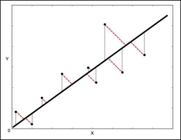
The Least square method calculates the error vertical to the line (shown by grey colour here) whereas ODR calculates the error perpendicular(orthogonal) to the line. This accounts for the error in both X and Y whereas using Least square method, we only consider the error in Y.
scipy.odr Implementation for Univariate Regression
import numpy as np
import scipy.odr.odrpack as odrpack
np.random.seed(1)

N = 100
x = np.linspace(0,10,N)
y = 3*x - 1 + np.random.random(N)
sx = np.random.random(N)
sy = np.random.random(N)

def f(B, x):
    return B[0]*x + B[1]
linear = odrpack.Model(f)
# mydata = odrpack.Data(x, y, wd=1./np.power(sx,2), we=1./np.power(sy,2))
mydata = odrpack.RealData(x, y, sx=sx, sy=sy)

myodr = odrpack.ODR(mydata, linear, beta0=[1., 2.])
myoutput = myodr.run()
myoutput.pprint()
 Output:

Beta: [ 3.02012861 -0.6316873 ]
Beta Std Error: [0.01188348 0.05616464]
Beta Covariance: [[ 0.00067276 -0.00267083]
 [-0.00267083  0.01502795]]
Residual Variance: 0.20990666070258754
Inverse Condition #: 0.10598108443798755
Reason(s) for Halting:
  Sum of squares convergence
SciPy optimize
Various commonly used optimization algorithms are included in this subpackage. It basically consists of the following:
- Unconstrained and constrained minimization of multivariate scalar functions i.e minimize (eg. BFGS, Newton Conjugate Gradient, Nelder_mead simplex, etc)
- Global optimization routines (eg. differential_evolution, dual_annealing, etc)
- Least-squares minimization and curve fitting (eg. least_squares, curve_fit, etc)
- Scalar univariate functions minimizers and root finders (eg. minimize_scalar and root_scalar)
- Multivariate equation system solvers using algorithms such as hybrid Powell, Levenberg-Marquardt.
Rosenbrock Function:
In mathematical optimization, the Rosenbrock function is a non-convex function, introduced by Howard H. Rosenbrock in 1960, which is used as a performance test problem for optimization algorithms. The function computed is:
sum(100.0*(x[1:] - x[:-1]**2.0)**2.0 + (1 - x[:-1])**2.0
where,
x is a 1-D array of points at which the Rosenbrock function is to be computed. It returns a float that is the value of the Rosenbrock function.Here is an example:
import numpy as np
from scipy.optimize import rosen
a = 2 * np.arange(3)
print(a)
rosen(a)
 Output:
[0 2 4]
402.0
Nelder-Mead:
The Nelder–Mead method (also downhill simplex method, amoeba method, or polytope method) is a commonly applied numerical method used to find the minimum or maximum of an objective function in a multidimensional space. In the following example, the minimize method is used along with the Nelder-Mead algorithm.
import numpy as np
import scipy
from scipy.optimize import minimize
#define function f(x)
def f(x):
    return .2*(1 - x[0])**2
x1=np.array([1.3, 0.7, 0.8, 1.9, 1.2])
scipy.optimize.minimize(f,x1, method="Nelder-Mead")
 Output:

final_simplex: (array([[0.99999193, 0.74219995, 0.85278502, 1.96410543, 1.22139255],
       [1.00001128, 0.74220272, 0.85278008, 1.96402033, 1.22142657],
       [0.99998629, 0.74218966, 0.85279934, 1.96405769, 1.22141367],
       [1.00001666, 0.74218124, 0.85279   , 1.9640668 , 1.22140094],
       [0.99998324, 0.74220839, 0.85280501, 1.96409484, 1.22137052],
       [1.00001953, 0.74218806, 0.85279976, 1.96412167, 1.22137807]]), array([1.30328312e-11, 2.54555652e-11, 3.75756702e-11, 5.54966943e-11,
       5.61852242e-11, 7.62918514e-11]))
           fun: 1.303283116723792e-11
       message: 'Optimization terminated successfully.'
          nfev: 136
           nit: 70
        status: 0
       success: True
             x: array([0.99999193, 0.74219995, 0.85278502, 1.96410543, 1.22139255])
So,the solution to the above problem is [0.99999193, 0.74219995, 0.85278502, 1.96410543, 1.22139255].
Another optimization algorithm that needs only function calls to find the minimum is Powell‘s method, which is available by setting method = 'powell' in the minimize() function.
Least Square Minimization
It is used to solve the nonlinear least-square problems bound on the variables. Given the residuals (difference between observed and predicted value of data) f(x) (an n-dimension real function of n real variables) and the loss function rho(s) (a scalar function), least_square finds a local minimum of the cost function f(x): Let's consider the following example:
from scipy.optimize import least_squares
import numpy as np
input = np.array([2, 2])
def rosenbrock(x):
   return np.array([10 * (x[1] - x[0]**3), (1 - x[0])])
res = least_squares(rosenbrock, input)
print(res)
 Output:

active_mask: array([0., 0.])
        cost: 0.0
         fun: array([0., 0.])
        grad: array([0., 0.])
         jac: array([[-30.00000045,  10.   ],
       [ -1.        ,   0.        ]])
     message: '`gtol` termination condition is satisfied.'
        nfev: 4
        njev: 4
  optimality: 0.0
      status: 1
     success: True
           x: array([1., 1.])
SciPy fsolve()
The scipy.optimize library provides the fsolve() function, which is used to find the root of the function. It returns the roots of the equation defined by fun(x) = 0 given a starting estimate. Consider the following example:
from scipy.optimize import fsolve
def func(x):
    return [x[0] * np.cos(x[1]) - 4,
            x[1] * x[0] - x[1] - 5]
root = fsolve(func, [1, 1])
root
 Output:
array([6.50409711, 0.90841421])
This brings us to the end of this article where we explored the wide variety of functions provided by the SciPy library. I would recommend going through the documentation to get a more in-depth knowledge of this library. Check out this SciPy course today.