
Time series analysis has been widely used for many
Parameters
Stationarity
Data attains stationarity when the properties such as average value, variation of the data, and standard deviation do not change over time. It is also an assumption to hold as the data which is not stationary can wrongly forecast results. Here’s an example:
If we look closely into the above diagrams, the left diagram clearly tells that the data has an upward trend but it is not stationary. The graph clearly shows that the mean over the different time periods is not the same and is rapidly fluctuating. On the other hand, if we look into the right one, the data has no trend. It moves over a straight line and has a constant mean and variance over different time periods. Hence, this type of data is suitable for analysis.
Seasonality
Data is said to be seasonal when it changes exactly in the same way over a different time period. Let us consider the following data.
If we look into the data, it contains the death toll of people from 2006 to 2016 i.e 10 years. Now we can see that the upward fluctuations occurred during the starting of every year and it came to a minimum during the mid-year period. This clearly implies that the death of these people follows a pattern and it can also be inferred that the death after the mid-year period is higher than the initial 6 months in every year. This is considered as another assumption of a time series data which needs to be true for successful forecasting.
Autocorrelation
This is another important parameter which assumes that the data needs to be auto-correlated. Data is said to be auto-correlated when it shows similar observations over a time lag present in the data.
Let’s take a closer look at the chart above. If we see the data, we see that the first value and the 24th value happen to be the same. Also, the 12th value and the 36th value happen to be the same. A quick inference? The graph implies that the data follows a high correlation as it is showing similar observations in every 24-hour period. Although it is quite difficult to get data with these types of correlation, we can hold an assumption that the data should be approximately correlated.
Take a look at this free resource for you to enhance your knowledge of time series: Time Series Analysis Stock Market Prediction Python.
Applications
Time series analysis can apply to many sectors including but not limited to:
- Power generation companies to observe the usage of electricity
- Financial sectors such as banking, stock market, etc.
- Weather forecasting to predict the weather.
- Traffic engineering to study traffic volume during peak hours.
- Forecasting hospital blood requirements
Types of time series analysis.
There are plenty of methods for time series analysis, some of them are:
- Moving Average method
- Exponential Smoothing
- Holt’s Winter Method
- ARIMA
- RNN (Recurrent Neural Network)
The first two types are often less used as they have limited capability when it comes to forecasting. RNN is a topic covered in deep learning. In this article, we will cover Holt’s Winter Method and ARIMA as these two are the most commonly used when it comes to time series analysis. Interestingly, moving average and exponential smoothing techniques are quite naïve and some of their traits are already present in ARIMA algorithm and Holt’s Winter method so we will mainly focus on those.
What is ARIMA?
ARIMA stands for Auto Regression Integrated Moving Average and is used to forecast time series following a seasonal pattern and a trend. It has three key aspects, namely:
- AR - Auto Regression or simply AR denotes a relationship between an observation and a lagged observation.
- I - Integration or I stands for the steps required to make the data stationary. One naïve step is to subtract an observation from one step previous observation thus making data stationary.
- MA- Moving Average or MA is an assumption that the model holds a relationship between an observation and the residuals of the moving average of the lagged observation.
It uses a linear regression technique to make future forecasting by making the data stationary in order to remove trend and seasonality which can affect the overall performance of the model.
Inclusive of its dynamic principle and its working process, it also considers three major parameters, failing which can lead to less intuitive forecasting.
- p- This parameter is also known as lag order which is defined as the number of lag observations present in the model.
- d- It is also known as the degree of differencing or simply defined as the steps that are required to make the data stationary.
- q- It is a window of moving average of the lagged observations and is also known as the order of moving average.
Applying ARIMA in Python
Let us code an ARIMA model in Python.
We will be using some data on monthly milk production. Let us import all the necessary libraries:
import numpy as np
import pandas as pd
import statsmodels.api as sm
import matplotlib.pyplot as plt
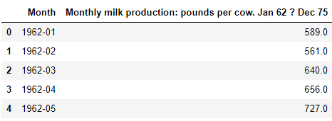
Now we will read the data and locate the head of it.
df = pd.read_csv(‘milk-production.csv')
df.head()
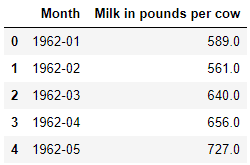
The columns names are a bit fuzzy. Let us change it up.
df.columns = ['Month','Milk in pounds per cow']
df.head()
Now it looks better.
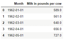
Next, let’s perform a time series analysis. It is often required or considered mandatory to change the dates to proper data types and in python, we can do that by using 'pd.datetime'.
df['Month'] = pd.to_datetime(df['Month'])
df.head()
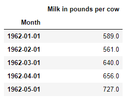
Now we will set the index to the date column.
df.set_index('Month',inplace=True)
df.head()
Now it is time to see the trend and seasonality of the data.
df.plot()
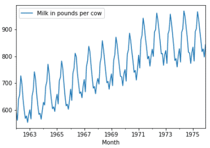
As we see the data tends to be following a seasonal pattern having an upward trend.
Now let us perform a rolling statistic to see the variation of the mean and standard deviation.
timeseries = df ['Milk in pounds per cow']
timeseries.rolling(12).mean().plot(label='12 Month Rolling Mean')
timeseries.rolling(12).std().plot(label='12 Month Rolling Std')
timeseries.plot()
plt.legend()
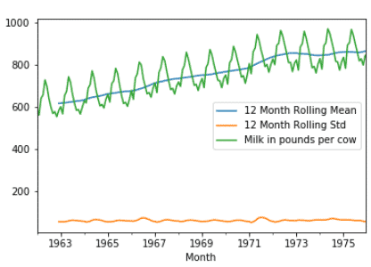
As we see, the mean (average) of milk production is trending linearly upward.
Now we will be seeing the seasonality trend and residuals by using ETS decomposition:
from statsmodels.tsa.seasonal import seasonal_decompose
decomposition = seasonal_decompose(df['Milk in pounds per cow'], freq=12)
figure = plt.figure()
figure = decomposition.plot()
figure.set_size_inches(15, 8)
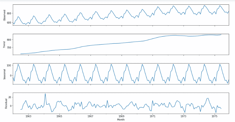
The data is indeed seasonal and follows an upward trend. Also, the average value or the mean of the residuals seem to be zero which holds our assumption.
Now we will check whether the data is stationary or not. For this, we will perform a test called the Dickey-Fuller test. In the field of statistics, the Dickey-Fuller test (ADF) is used to test the null hypothesis, i.e. to check if a unit root is present in a sample of a time-series data. The alternative hypothesis is considered to be different on the version we use but is usually considered stationarity or trend-stationarity.
Basically, we are trying to decide whether to accept the Null Hypothesis or go with the Alternative Hypothesis (that the time series has no unit root and is stationary).
We end up deciding this based on the return of the p-value.
A small p-value which is considered below 0.05 indicates strong evidence against the null hypothesis, thereby we reject the null hypothesis.
A large p-value which is considered above 0.05 indicates weak or no evidence against the null hypothesis, thereby we fail to reject the null hypothesis.
Let's run the test:
from statsmodels.tsa.stattools import adfuller
test_result = adfuller(df['Milk in pounds per cow'])
print ('ADF Test:')
labels = ['ADF Statistic','p-value','No. of Lags Used','Number of Observations Used']

for value,label in zip(test_result,labels):
    print (label+’: '+str(value))
if test result [1] <= 0.05:
    print ("Reject null hypothesis and data is stationary")
else:
    print ("Fail to reject H0 thereby data is non-stationary ")
After running the above function, we get the following output.
'ADF Test:'
'ADF Statistic': -1.30381158742
p-value: 0.627426708603
No. of Lags Used: 13
Number of Observations Used: 154
   Fail to reject H0 thereby data is non-stationary
Now we will build a function for further use to check the stationarity of the data
# Store in a function for later use!
def check_adf(time_series):
    test_result = adfuller(time_series)
    print (ADF Test:')
    labels = ['ADF Statistic','p-value','No. of Lags Used','Number of Observations Used']
    for value,label in zip(test_result,labels):
        print (label+’: '+str(value))
    if test result [1] <= 0.05:
        print ("Reject null hypothesis and data is stationary")
    else:
        print ("fail to reject H0 and data is non-stationary ")
Now it is clear that the data is non-stationary so we need to apply differencing to make our data stationary.
We have realised that our data is seasonal (it is also pretty obvious from the plot itself). This means we need to use Seasonal ARIMA on our model. If our data was not seasonal, it means we could have used just ARIMA on it. We will take this into account while differencing our data.
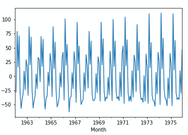
Now let us do our first difference.
df ['Milk First Difference'] = df ['Milk in pounds per cow'] - df ['Milk in pounds per cow']. shift (1)
adf_check(df['Milk First Difference'].dropna())
After performing the above step, we get the following output:
ADF Test:
ADF Statistic: -3.05499555865
p-value: 0.0300680040018
No. of Lags Used: 14
Number of Observations Used: 152
Reject null hypothesis and data is stationary
So, by doing the first difference we made our data stationary. Sometimes, we need to do more differencing in order to make our data stationary.
df ['Milk First Difference']. plot ()
Now we will check how autocorrelation works in the data by importing library to implement ACF plot.
from statsmodels.graphics.tsaplots import plot_acf
fig_first = plot_acf(df["Milk First Difference"].dropna())
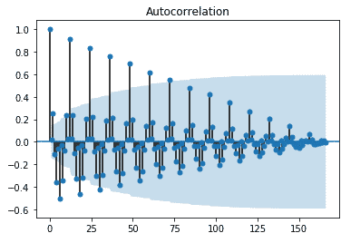
We can see that the data is showing similar fluctuations in the lagged observations which confirm that they are correlated.
Now it's time to perform ARIMA.
Please note we have seasonal data! So, we will use SARIMA
model = sm.tsa.statespace.SARIMAX(df['Milk in pounds per cow'],order=(0,1,0), seasonal_order=(1,1,1,12))
ARIMAresult = model.fit()
print (ARIMAresult.summary())
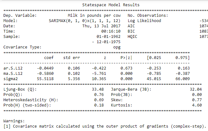
Here the main thing to observe is the AIC which should be minimum. To improve our model, we can play around changing the p,d,q parameters and the model which gives the least AIC is the best model.
Now let us predict the future values to see how it performs.
df['forecast_data'] = ARIMAresult.predict(start = 150, end= 168, dynamic= True)
df [['Milk in pounds per cow','forecast_data']]. plot (figsize= (12,8))
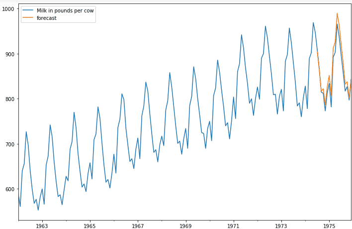
As we can see, the model is performing just the way we expected.
Applying ARIMA in R
We have seen how time series using ARIMA works in Python. Now we can see how it works in R.
For R, we will be using a restaurant dataset which contains data of visitors in a restaurant during a particular time period.
df_air <- read_csv (file = '../input/recruit-restaurant-visitor-forecasting/air_visit_data.csv')
df_air_store <- read_csv('../input/recruit-restaurant-visitor-forecasting/air_store_info.csv')
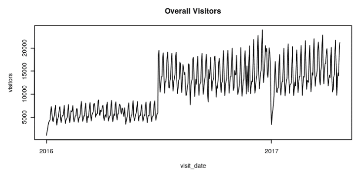
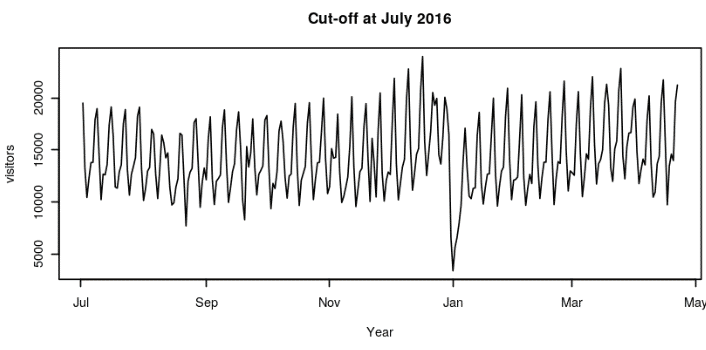
From the above diagram, we can infer that there is a strong increase in the number of visitors from mid-2016 and it is hard to verify the cause of such an increase. So, we will take the data from July 2016.
Now we will fit an ARIMA model to predict visitors who visited the restaurant from February 2017 and see how it performs.
merged_train <- merged_sum %>% filter (visit_date <='2017-02-01')
merged_test <- merged_sum %>% filter (visit_date >'2017-02-01')

#print(paste(nrow(merged_sum), nrow(merged_train), nrow(merged_test)))
m <- arima(merged_train$visitors, order=c(2,1,2), seasonal= list(order=c(1,1,1), period=7))
y_prediction <- forecast: forecast (m, h=80)
par (mfrow=c (1,1), cex=0.7)
plot(ts(merged_sum$visitors), main="ARIMA model predictions, cut off at Feb 2017")
lines (y_prediction$mean, col='red')
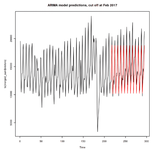
Now after fitting, we have come to see that the model just performs how we expected. However, we can play around with the parameters such as order and period to see any further improvements.
Holt’s Winter Method - An Overview
Holt’s Winter method is a type of exponential smoothing technique which is used to forecast for a shorter time period by either using additive or multiplicative approach over a particular trend and seasonality. The parameters used for smoothing in this method are alpha, beta and gamma which have following functions
- The alpha parameter is used as a smoothing factor for the level.
- The beta parameter is used to perform exponential smoothing to the data having trend. To perform the same, we must set it to FALSE.
- The gamma parameter is used for components having seasonality. If we set it to FALSE, the model fitted will be non-seasonal.
Holt’s winter method is determined based on the nature of the data and its seasonal pattern. If the seasonality tends to be linear, we use the additive seasonality approach. If the seasonality tends to be exponential, we use the multiplicative seasonality approach.
Applying Holt’s Winter method in R
We will be implementing Holt’s Winter method in R. The data we will use is monthly sales data which consists of sales figures for a particular day and we need to forecast for the next 12 months.
Let us import the following libraries:
library(readr)
library(dplyr)
library(ggplot2)
library(forecast)
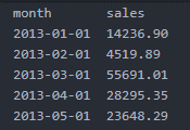
Let us read and check the head of the data
df <- read_csv("../input/MonthlySales.csv")
Now let us check the first five rows
head (df, n = 5)
Now let us plot the data to see the trend and seasonality.
options (repr.plot.width = 6, repr.plot.height = 3)
ggplot(df, aes(x = month, y = sales)) + geom_line() + geom_smooth(method = 'lm') +labs(x = "Time", y = "Monthly Sales")
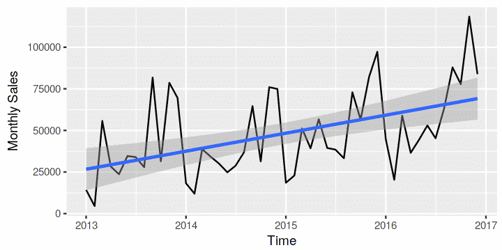
Looking closely, the data is trending upward and it has seasonality which is extending in a linear fashion. So, we will use the additive model for this data.
Now we will observe trend and seasonality individually by using decomposition plot. For that, we need to convert the sales column to a time series object.
New_sale<- ts(df$sales, frequency = 12, start = c(2013,1))
class (New_sale)
Let us see the decomposition plot:
options (repr.plot.width = 6, repr.plot.height = 5)
salesDecomp_plot <- decompose (New_sale)
plot(salesDecomp_plot)
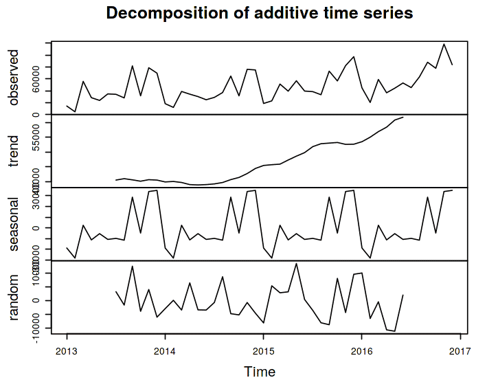
The data follows an upward trend and it also has a seasonal pattern. Now it's time to build the model.
Sales_Log <- log (New_sale)
HW_model <- HoltWinters(Sales_Log)
HW_model
After fitting the model, let us visualise to see how did it perform.
options (repr.plot.width = 6, repr.plot.height = 4)
plot (HW_model)
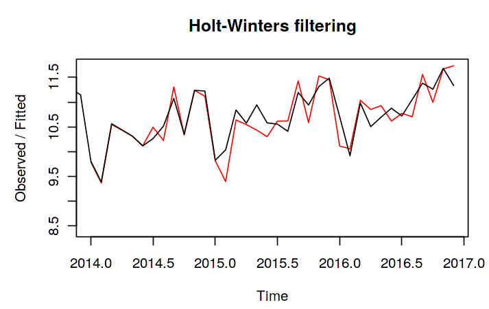
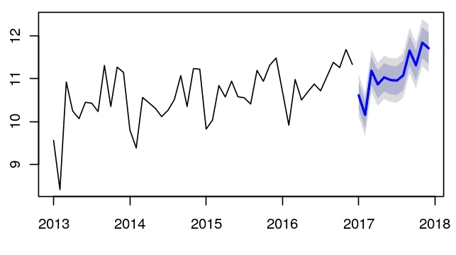
Well, the model performed exceptionally well as the observed values and the fitted values match closely. So hopefully, it won’t fail in prediction. Let us do that. We will predict for the next 12 months.
Forecast_sales <- forecast (HW_model, h=12)
# plot
plot (Forecast_sales)
Inference
ARIMA can deal with any time series analysis as it makes the data stationary first, but it is not the case in Holt’s Winter method. Holt’s Winter method considers that the data must have a trend and seasonality. Nevertheless, the error in prediction is more compared to ARIMA. Mostly the real-world data such as stock market data which are quite difficult to analyse often use deep learning techniques such as RNN, LSTM, etc.
If you wish to learn more about time series analysis and other concepts of data science and analytics, upskill with Great Learning's PG program in Data Science.
Explore endless possibilities with our comprehensive selection of free courses. Whether you're interested in Cybersecurity, Management, Cloud Computing, IT, or Software, Artificial Intelligence and Machine Learning, we have the perfect industry-relevant domain for you. Gain the essential skills and expertise needed to excel in your desired field.