In this guide, we are going to show you exactly how AdaBoost works, step-by-step.
We are going to cover:
- The mathematical formulas behind the algorithm.
- The concept of "Weak Learners" and Decision Stumps.
- The critical "Weight Update" and "Bucketing" mechanisms.
- How to implement it in Python.
Let's dive into mastering this fundamental Machine Learning technique.
What is AdaBoost?
AdaBoost (short for Adaptive Boosting) is a supervised machine learning algorithm used for classification.
It is part of a family of algorithms known as Ensemble Methods.
But here is the thing that makes AdaBoost unique:
Unlike Random Forest, which builds trees in parallel (Bagging), AdaBoost builds models sequentially (Boosting).
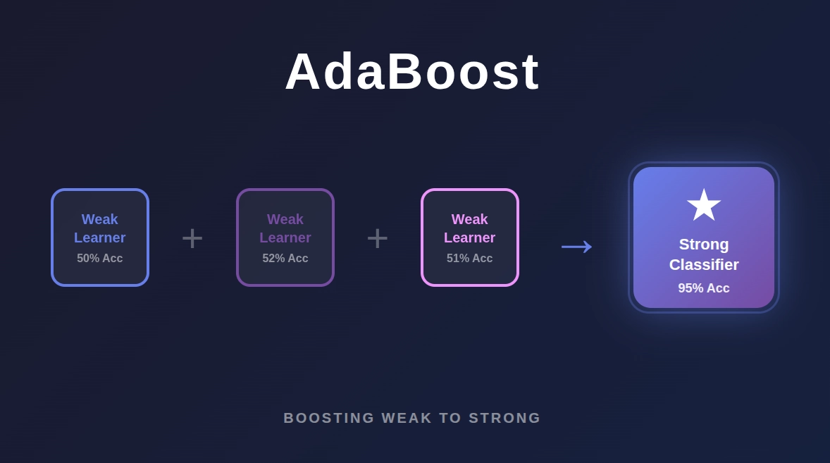
It converts a set of "Weak Learners" into a single "Strong Learner."
The Core Concept: "Adaptive" Learning
Why is it called Adaptive?
Because the algorithm adjusts itself after every iteration.
- It builds a model.
- It identifies the errors (misclassified data).
- It adapts by assigning higher weights to those errors.
- The next model focuses exclusively on fixing those errors.
This iterative process reduces bias, allowing the model to capture complex patterns that a single Decision Tree would miss.
The "Bias vs. Variance" Trade-off
To understand why AdaBoost is so effective, you need to understand the two main sources of error in Machine Learning:
- Bias: Error caused by overly simple assumptions (underfitting).
- Variance: Error caused by too much complexity (overfitting).
AdaBoost is unique because it focuses on reducing Bias. Unlike Random Forest, which builds deep trees in parallel to reduce variance, AdaBoost builds shallow stumps sequentially to aggressively fix errors.
Learn Machine Learning with Python
Learn machine learning with Python! Master the basics, build models, and unlock the power of data to solve real-world challenges.
The Architecture (Decision Stumps)
To understand AdaBoost, you first need to understand the Decision Stump.
Most people think AdaBoost uses Decision Trees. That is technically true, but they are not the deep trees you see in a Random Forest.
They are Stumps.
A Decision Stump is a tree with a max_depth of 1.
- It has one root node.
- It has two leaf nodes.
- It performs a single split on a single feature.
This is the definition of a Weak Learner. A stump is only slightly better than random guessing.
However, AdaBoost combines hundreds or thousands of these stumps to create a highly accurate prediction engine.
How AdaBoost Works (The Step-by-Step Process)
This is the most important part of the guide.
We are going to walk through the exact mathematical process AdaBoost uses to train a model.
Let’s imagine we have a dataset with 5 records (Samples).
Step #1: Assign Initial Weights
When the algorithm starts, every sample is equal.
We assign a Sample Weight (w) to every row in the dataset using this formula:

Where N is the total number of records.
Since we have 5 records, every row starts with a weight of 0.2.
Step #2: Create the First Base Learner
The algorithm looks at all the features and creates the first Decision Stump.
It selects the stump that has the lowest Gini Impurity or Entropy.
Let's say Stump 1 predicts 4 records correctly and 1 record incorrectly.
Step #3: Calculate the Total Error (TE)
This is where many people get confused.
The Total Error is not just the number of wrong guesses. It is the sum of the weights of the misclassified samples.
Since the weight of our one wrong record is 0.2:
TE = 0.2
Step #4: Calculate "Amount of Say" (Alpha)
Now we need to calculate how important this stump is. This is called the Amount of Say (denoted by Alpha, α).
We use this formula:
Let’s plug in our error (0.2):
- (1 - 0.2) / 0.2 = 4
- ln(4) ≈ 1.386
- 0.5 × 1.386 ≈ 0.693
So, the Alpha (α) for this stump is 0.693.
The Key Takeaway:
- Low Error: High Alpha (Positive). The stump has a strong vote.
- High Error (0.5): Zero Alpha. The stump has no vote.
- Random Guessing: If error is 50%, the stump is useless.
Step #5: Update the Weights
This is the "Boosting" part. We need to tell the next stump which records are difficult.
We update the weights for incorrectly classified records using this formula:
Since α is positive, eα is greater than 1.
Result: The weight increases.
We update the weights for correctly classified records using this formula:
Result: The weight decreases.
Step #6: Normalize the Weights
After the update, the weights will no longer sum up to 1. To fix this, we divide every weight by the sum of the new weights.
Now, the difficult record (the one we got wrong) has a much higher probability (weight) than the easy records.
Step #7: The Bucket Method (Resampling)
This is the mechanism AdaBoost uses to pass the data to the next learner.
We create a new dataset of size N (5 records) by resampling the original data.
We use the Bucket Method:
- We create "buckets" based on the normalized weights.
- The record with the high weight gets a large bucket (e.g., from 0.0 to 0.50).
- The records with low weights get tiny buckets (e.g., from 0.50 to 0.55).
- We pick a random number between 0 and 1.
Because the difficult record has a massive bucket, the random number will likely fall inside it multiple times.
The Result: The new dataset contains multiple copies of the difficult record.
When the next Decision Stump tries to minimize errors on this new dataset, it must classify that difficult record correctly, or its error rate will be huge.
Making the Final Prediction
Once we have trained all our stumps (let's say 50 of them), how do we make a prediction on test data?
We use a Weighted Majority Vote.
We calculate the prediction for a new data point, x, using this sign function:
Here is what happens in plain English:
- Every stump makes a prediction (+1 or -1).
- We multiply each prediction by that stump's Alpha (α).
- We sum them all up.
- If the result is positive, we predict Class 1. If negative, Class -1.
This ensures that the "smart" stumps (high Alpha) count more than the "weak" stumps.
Python Implementation
Implementing AdaBoost is straightforward using the scikit-learn library.
Here is a clean, production-ready code snippet.
from sklearn.ensemble import AdaBoostClassifier
from sklearn.tree import DecisionTreeClassifier
from sklearn.datasets import make_classification
from sklearn.model_selection import train_test_split
from sklearn.metrics import accuracy_score

# 1. Generate a sample dataset
X, y = make_classification(n_samples=1000, n_features=20, random_state=42)
X_train, X_test, y_train, y_test = train_test_split(X, y, test_size=0.3)

# 2. Define the Weak Learner (Stump)
# We strictly set max_depth to 1
stump = DecisionTreeClassifier(max_depth=1, max_features='auto')

# 3. Initialize AdaBoost
# n_estimators: The number of stumps to create
# learning_rate: Controls the contribution of each model
ada = AdaBoostClassifier(
    base_estimator=stump,
    n_estimators=50,
    learning_rate=1.0,
    algorithm='SAMME'
)

# 4. Fit the model
ada.fit(X_train, y_train)

# 5. Evaluate
predictions = ada.predict(X_test)
print(f"Model Accuracy: {accuracy_score(y_test, predictions)}")
Key Hyperparameters
n_estimators: The number of stumps. Increasing this generally improves performance but increases training time.learning_rate: This shrinks the contribution of each tree. There is a trade-off: if you lower the learning rate, you usually need to increasen_estimators.
Pros and Cons
AdaBoost is powerful, but it is not a silver bullet. You need to know when to use it.
The Advantages
- High Accuracy: It pushes the limits of weak learners.
- No Parameter Tuning: Compared to SVM or Neural Networks, AdaBoost works well "out of the box."
- Feature Selection: It implicitly identifies important features by ignoring irrelevant ones during stump creation.
The Disadvantages (The Pain Point)
There is one major issue you must be aware of: Outliers.
Because AdaBoost minimizes the Exponential Loss Function, it applies massive weights to misclassified samples.
If your dataset has noisy outliers (garbage data), AdaBoost will obsess over them. It will ruin the model by trying to fit points that shouldn't be fitted.
Pro Tip: If your data is noisy, use Gradient Boosting or Random Forest instead. They are more robust to noise.
Conclusion
AdaBoost is a fundamental algorithm in the Machine Learning ecosystem.
It introduced the world to the power of Boosting: the idea that many weak models can combine to become a master predictor.
It works by:
- weighting errors,
- calculating performance (Alpha),
- and resampling data via buckets.
If you have clean data and need a fast, accurate classifier, AdaBoost is an excellent choice.
Our Machine Learning Courses
Explore our Machine Learning and AI courses, designed for comprehensive learning and skill development.
| Program Name | Duration |
|---|---|
| MIT No Code AI and Machine Learning Course | 12 Weeks |
| MIT Data Science and Machine Learning Course | 12 Weeks |
| Data Science and Machine Learning Course | 12 Weeks |