Apache Spark

Intro to Spark
What is Spark
About Apache Spark
Why Spark
What is Scala
Functional Programming
Spark Vs Hadoop
Spark Architecture
Spark Deployment Modes
RDDs
RDDs Operations
Immutability
Lazy Evaluation
Type Inference
Caching
Loading spark data objects (RDD)
RDD Properties
How to create RDD in spark
How is the data stored in RDD
RDD Drawbacks
Spark Dataframe
Spark Datasets
Actions and transformations
Spark SQL
Spark Runtime Architectures
Pyspark code – Hands on

Spark Intro:

Spark is another parallel processing framework. However, just not yet another parallel processing framework, Hadoop for example, what we have been seen all this while was a very popular parallel processing framework but it had actually had a lot of shortcomings especially in the area of machine learning, Hence a lot of those shortcomings of Hadoop was addressed and all-new parallel processing frameworks was designed and that is actually called Spark.

Yes, Spark sounds like an actual spark into the life where it has made a lot of tasks made much easier.

What is Spark?

Apache Spark is a fast, in-memory data processing engine
With development APIs, it allows executing streaming, machine learning or SQL.
Fast, expressive cluster computing system compatible with Apache Hadoop
Improves efficiency through:
- In-memory computing primitives
- General computation graphs (DAG)
- Up to 100× faster
Improves usability through:
- Rich APIs in Java, Scala, Python
- Interactive shell
- Often 2-10× less code
open-source parallel process computational framework primarily used for data engineering and analytics.

About Apache Spark:

Initially started at UC Berkeley in 2009
Open source cluster computing framework
Written in Scala (gives the power of functional Programming)
Provides high-level APIs in
- Java
- Scala
- Python
- R
Integration with Hadoop and its ecosystem and can read existing data.
Designed to be fast for iterative algorithms and interactive queries for which MapReduce is inefficient.
Most popular for running Iterative Machine Learning Algorithms.
With support for in-memory storage and efficient fault recovery.
- 10x (on disk) – 100x (In-Memory) faster

Why Spark?

Most of Machine Learning Algorithms are iterative because each iteration can improve the results
With Disk-based approach each iteration output is written to disk making it slow

What is Scala?

A high-level programming language
Supports the functional style of programming
Supports OO-style of programming
It’s actually a multi-paradigm language

What is functional programming?

Consider the following code snippet

int a = 10; //A new variable “a” is getting created

a++ ; // We are incrementing the variable a

Print(a) // will generate 11 as the o/p

Consider another way of doing the same thing

int a= 10;

int a1 = a + 1 ; // We are creating a new variable a1

Print(a) ; // a will still contain the value 10, state of the //variable a is not changed.

What is happening behind the scenes here?

An object or a variable, ‘a’ was actually created and the value called 10 was allocated and it is got stored in the memory.

When I increment the value which I stored in the variable “a” by using the operator “a++” which is very common in c or c++ style of programming, what eventually happens is in the same memory location the value will get incremented, meaning we are changing the value of the original variable. So what do we say here is like the state of the variable is changing actually in the course of the program execution.

Functional Programming:

Functional style of programming inherently supports parallelism

Functional style of programming is not restricted to a particular programming language.

It can be implemented in any language, just like the way OO concepts can also be implemented in a programming language like C

Certain programming languages inherently support the functional style of programming reducing the programmer’s burden

Scala is one of the functional programming languages

Spark in comparison to Hadoop:

Now let us try to compare Spark to Hadoop and is the easiest way to understand Spark.

However, a lot of things are very different in Spark and we will learn as go forward.

The high-level architecture of SPARK is very similar to that of HADOOP. Just like you have the Master-slave architecture, several data nodes and certain master nodes and is almost the same in Spark.
A quick way of understanding SPARK is by comparing it with HADOOP
Several drawbacks of Hadoop are addressed in Spark which gives a 10x-100x performance improvement over Hadoop
It is well suited for interactive and real time analytics of big data and streaming data
Its highly popular among machine learning users since it outperforms Hadoop in iterative workloads. This is because the framework itself facilitates to work better on iterative workloads, whereas the Hadoop framework does not hold good for iterative workloads because of intensive disk I/O operations(which is behind the scenes in Hadoop ecosystem)

Here certain mechanisms are actually put in place in spark to minimize the disk I/O operations.

Let us know some interesting facts but not myths:

The common myth around spark is that Spark is 10x/100x faster when compared to Hadoop because of completely in-memory based architecture, which is false.

It is not completely in memory architecture. There are also situations where disk I/O operations become inevitable but what to be kept in the memory and how long the results can be kept in the memory is completely under the control of programmer here in the case of Spark, thereby making it very favourable to gain increased performance when compared to Hadoop.

In this way, Spark is advanced but not completely in-memory based computing architecture.

In Hadoop, we basically have the data nodes to work in the slave mode and then they have the active name nodes, standby name nodes, and secondary name node and then we have the resource manager which does the work of the job tracker when compared to Hadoop version 1 and then the centralized scheduling and resource allocation actually happens with the help of resource manager scheduler in conjunction with the node manager and per application, application master in your datanodes.

Now let us have a quick recap of job execution in Hadoop:

Overview of job execution in Hadoop:

A job submitted by the user is picked up by the name node and the resource manager

The job gets submitted to the name node and eventually, the resource manager is responsible for scheduling the execution of the job on the data nodes in the cluster

The data nodes in cluster consist of the data blocks on which the user’s program will be executed in parallel

Driver is the starting point of a job submission (this can be compared to the driver code in Java MR)
Cluster Manager can be compared to the Resource Manager in Hadoop
Worker nodes are the data nodes in a HADOOP cluster
The executor can be compared to that of a node manager in Hadoop 2 or task tracker in Hadoop 1

Spark Deployment modes:

Standalone (used for learning & development)
- This is very similar to the pseudo-distributed mode of Hadoop
- Spark services run on multiple JVM’s
- This is also known as a standalone cluster

Local mode (used for learning & development)
- There is a single JVM (no need of HDFS)

Cluster mode (can work with MESOS or YARN)
- Used for production environment & it’s a fully distributed mode

In Map stage, it will have a record reader and then a mapper, then in-memory sort operation ad the output of this will be fed to the Reduce stage, in which it has a stage called merge, where the output of multiple mapper machines are going to be merged as in they have arrived, then after merging they are going to be subject to the shuffle operation or an aggregation operation, after which the reducer logic which is written by the programmer, depending upon the problem statement and will be implemented in the reduce stage.

The final output will be written on to the HDFS as per the above block diagram.

The above example demonstrates a map-reduce job involving 3 mappers on 3 input splits
There is 1 reducer
Each input split on each data resides on the hard disc. Mapper reading them would involve a disc read operation.
There would be 3 disc read operations from all the 3 mappers put together
Merging in the reduce stage involves 1 disc write operation
Reducer would write the final output file to the HDFS, which indeed is another disc write operation
Totally there are a minimum of 5 disc I/O operations in the above example (3 from the map stage and 2 from reduce stage)
The number of disc read operations from the map stage is equal to the number of input splits

Calculating the number of disc I/O operations on a large data set:

Typically an HDFS input split size would be 128 MB
Let’s consider a file of size 100TB and the number of file blocks on HDFS would be (100 * 1024 * 1024) / 128 = 8,19,200
There would around 8.2 lakh mappers which needs to run on the above data set once a job is launched using Hadoop MapReduce
8.2 lakh mappers mean, 8.2 lakh disc read operations
Disc read operations are 10 times slower when compared to a memory read operation
Map-Reduce does not inherently support iterations on the data set
Several rounds of Map-Reduce jobs needs to be chained to achieve the result of an iterative job in Hadoop
Most of the machine learning algorithms involves an iterative approach
10 rounds of iterations in a single job leads to 8.2 lakh X 10 disc I/O operations

Spark’s approach to problem-solving:

Spark allows the results of the computation to be saved in the memory for future re-use
Reading the data from the memory is much faster than that of reading from the disc
Caching the result in memory is under the programmer’s control
Not always is possible to save such results completely in memory especially when the object is too large and memory is low
In such cases, the objects need to be moved to the disc
Spark, therefore is not completely in memory-based parallel processing platform
Spark, however, is 3X to 10X faster in most of the jobs when compared to that of Hadoop

Let us now see the major differences between Hadoop and Spark:

In the left-hand side, we see 1 round of MapReduce job, were in the map stage, data is being read from the HDFS(which is hard drives from the data nodes) and after the reduce operation has finished, the result of the computation is written back to the HDFS. Immediately if result produces by a particular MapReduce job has to be consumed by another MapReduce job. Once again the second mapper in the bottom have to read the data from the HDFS cluster which again involves a disk read operation from the hard drives of your data nodes and once again the result of the computation in the reduce stage will be written back to the HDFS

Now, in the right-hand side, we can see a Spark job meaning we have a map operation, then we have a reduce operation and then the result of map and join will be cached in memory. So there is no disk write operation involved over here immediately this can be fed as an input to the next job which might involve something like a map or something like a reduce or in this particular example, there is a transform operation happening here, so here we are eliminating a disk write operation.

In this example, we are eliminating 1 disk write operation. So caching plays a very important role in speeding up the computations when it comes to a spark ecosystem. But remember, Spark is not a completely in-memory data computation framework if this cache data is too large to fit in the memory, eventually we will have to force into the written on to the disk but we will try to keep that as many as possible and we will see how we can achieve this and will go deeper into this part down the line.

What Spark gives Hadoop?

Machine learning module delivers capabilities not easily exploited in Hadoop.
in-memory processing of sizeable data volumes remains an important contribution to the capabilities of a Hadoop cluster.
Valuable for enterprise use cases
- Spark’s SQL capabilities for interactive analysis over big data
- Streaming capabilities (Spark streaming)
- Graph processing capabilities (GraphX)

What Hadoop gives Spark?

YARN resource manager
DFS
Disaster Recovery capabilities
Data Security
A distributed data platform
Leverage existing clusters
Data locality
Manage workloads using advanced policies
- Allocate shares to different teams and users
- Hierarchical queues
- Queue placement policies
Take advantage of Hadoop’s security
- Run-on Kerberized clusters

Driver is the starting point of a job submission (this can be compared to the driver code in Java MR)
Cluster Manager can be compared to the Resource Manager in Hadoop
Worker is a software service running on slave nodes, similar to the are the data nodes in a HADOOP cluster
The executor is a container which is responsible for running the tasks

Spark Deployment Modes:

Standalone mode :

All the spark services run on a single machine but in separate JVM’s. Mainly used for learning and development purposes(something like the pseudo-distributed mode of Hadoop deployment)

Cluster mode with YARN or MESOS:

This is the fully distributed mode of SPARK used in a production environment

Spark in Map Reduce (SIMR) :

Allows Hadoop MR1 users to run their MapReduce jobs as spark jobs

RDDs:

Key Spark Construct
A distributed collection of elements
Each RDD is split into multiple partitions which may be computed on different nodes of the cluster
Spark automatically distributes the data in RDD across cluster and parallelize the operations
RDD has the following properties
- Immutable
- Lazy evaluated
- Cacheable
- Type inferred

RDDs as an advantage:

They are objects in SPARK which represent BIG DATA
They are distributed
They are fault-tolerant
They are lazily evaluated
Scalable
Supports near real-time stream processing
They have a lot of other benefits which makes it THE element of BIG DATA computation in SPARK

RDD Operations:

How to create RDD:
- Loading external data sources
  - lines=sc.textfile(“readme.txt”)
- Parallelizing a collection in a driver program
  - Lines=sc.parallelize([“pandas”, “I like pandas”])
Transformation
- transform RDD to another RDD by applying some functions
- Lineage graph (DAG): keep the track of dependencies between transformed RDDs using which on-demand new RDDs can be created or part of persistent RDD can be recovered in case of failure.
- Examples : map, filter,flapmap,distinct,sample , union, intersect,subtract ,cartesian etc.
Action
- Actual output is being generated in transformed RDD once the action is applied
- Return values to the driver program or write data to external storage
- The entire RDD gets computed from scratch on new action call and if intermediate results are not persisted.
- Examples : reduce, collect,count,countByvalue,take,top,takeSample,aggreagate,foreach etc.

Immutability:

Immutability means once created it never changes
Big data by default immutable in nature
Immutability helps to
- Parallelize
- Caching

Immutability in action

const int a = 0 //immutable

int b = 0; // mutable

Updation

b ++ // in place

c = a + 1

Immutability is about value not about reference.

Challenges of Immutability:

Immutability is great for parallelism but not good for space

Doing multiple transformations result in

○ Multiple copies of data

○ Multiple passes over data

In big data, multiple copies and multiple passes will have poor performance characteristics

Lazy Evaluation:

Laziness means not computing transformation till it’s need
Once, any action is performed then the actual computation starts
A DAG (Directed acyclic graph) will be created for the tasks
Catalyst Engine is used to optimize the tasks & queries
It helps reduce the number of passes
Laziness in action

val c1 = collection.map(value => value +1) //do not compute anything

val c2 = c1.map(value => value +2) // don’t compute

print c2 // Now transform into

Multiple transformations are combined to one

val c2 = collection.map (value => {var result = value +1

result = result + 2 } )

Challenges of Laziness:

Laziness poses challenges in terms of data type
If laziness defers execution, determining the type of the variable becomes challenging
If we can’t determine the right type, it allows having semantic issues
Running big data programs and getting semantics errors are not fun.

Type Inference:

Type inference is part of the compiler to determine the type by value
As all the transformation are side effect free, we can determine the type by operation
Every transformation has a specific return type
Having type inference relieves you think about representation for many transforms.
Example:
- c3 = c2.count( ) // inferred as Int
- collection = [1,2,4,5] // explicit type Array

Caching:

Immutable data allows you to cache data for a long time
Lazy transformation allows recreating data on failure
Transformations can also be saved
Caching data improves execution engine performance
Reduces lots of I/O operations of reading/writing data from HDFS

Loading spark data objects (RDD)

The data loaded into a SPARK object is called as an RDD
A detailed discussion about RDD’s will be covered shortly

Under the hood:

Job execution starts with loading the data from a data source (e.g. HDFS) into spark environment
Data read from the hard drives of worker nodes and loaded into the RAM of multiple machines
The data could be spread out into different files (each file could be a block in HDFS)
After the computation, the final result is captured

Partitions and data locality:

Loading of the data from the hard drives to the RAM of the worker nodes is based on data locality
The data in the data blocks is illustrated in the block diagram below

RDD properties:

We have just understood 3 important properties of an RDD in spark

1) They are immutable

2) They are partitioned

3) They are distributed and spread across multiple nodes in a machine

Workflow:

RDD Lazy evaluation:

Lets start calling these objects as RDD’s hereafter
RDD’s are immutable & partitioned
RDD’s mostly reside in the RAM (memory) unless the RAM (memory) is running of space

Execution starts only when Action starts:

RDDs are fault-tolerant(resilient)

RDD’s lost or corrupted during the course of execution can be reconstructed from the lineage

Create Base RDD

Increment the data elements
Filter the even numbers
Pick only those divisible by 6
Select only those greater than 78

Lineage is a history of how an RDD was created from it’s parent RDD through a transformation
The steps in the transformation are re-executed to create a lost RDD

RDD properties:

They are RESILIENT DISTRIBUTED DATA sets
Resilience (fault tolerant) due to the lineage feature in SPARK
They are distributed and spread across many data nodes
They are in-memory objects
They are immutable

Spark’s approach to problem solving:

Spark reads the data from the disc once initially and loads it into its memory
The in-memory data objects are called RDD’s in spark
Spark can read the data from HDFS where large files are spit into smaller blocks and distributed across several data nodes
Data nodes are called as worker nodes in Spark eco system
Spark’s way of problem solving also involves map and reduce operations
The results of the computation can be saved in memory in case if its going to be re-used as the part of an iterative job
Saving a SPARK object(RDD) in memory for future re-use is called caching

Note : RDD’s are not always cached by default in the RAM (memory). They will have to be written on to the disc when the system is facing a low memory condition due to too many RDD’s already in the RAM. Hence SPARK is not a completely in memory based computing framework

3 different ways of creating an RDD in spark:

Created by read a big data file directly from an external file system, this is used while working on large data sets
Using the parallelize API, this is usually used on small data sets
Using the makeRDD API

Example:

The parallelize() method

sc = SparkContext.getOrCreate()

myrdd = sc.parallelize([1,2,3,4,5,6,7,8,9])

Data source API (eg. The textFile API)

sc = sc.textFile(“FILE PATH”)

How is the data stored in an RDD?

What is the data format inside an RDD?

It’s just raw sequence of bytes. Especially when its created using a

the textFile() or parallelize() API

Creating RDD’s using structured data (CSV data)

sc = sc.textFile(“sample.csv”)

myrdd = sc.flatMap(lambda e:e.split(” “))

myrdd.collect()

Drawbacks of RDDs:

They store data as a sequence of bytes
This suits unstructured data manipulation
Data does not have any schema
There is no direct support to handle structured data
The native API’s on RDD’s seldom provide any support for structured data handling
Special RDD format is needed to store structured data (BIG DATA)
A special set of API’s are needed to manipulate and query such RDD’s

Schema RDDs(Data frames)

The idea of named columns and schema for the RDD data is borrowed from data frames
Spark allows creation of data frames using specific data frame API’s
An RDD can be created using the standard set of regular data set API’s , schema can be assigned to the data and explicitly converted into a data frame
There is provision to manipulate the spark data frames using the library “SPARK SQL”
The standard set of SPARK transformation API’s can also be used on SPARK data frames

Creating a Spark Data frame:

Consider the following CSV data saved in a text file

1,Ram,48.78,45

2,Sita,12.45,40

3,Bob,3.34,23

4,Han,16.65,36

5,Ravi,24.6,46

rdd = sc.textFile(“sample.csv”)

csvrdd = rdd.map(lambda e:e.split(“,”))

emp = csvrdd.map(lambda e: Row( id=long(e[0]), name=e[1],sal=e[2], age=int(e[3].strip())))

empdf = sqlContext.createDataFrame(emp)

Dataframes in Spark:

Unlike an RDD, data is organized into named columns.
Allows developers to impose a structure onto a distributed collection of data.
Enables wider audiences beyond “Big Data” engineers to leverage the power of distributed processing
allowing Spark to manage the schema and only pass data between nodes, in a much more efficient way than using Java serialization.
Spark can serialize the data into off-heap storage in a binary format and then perform many transformations directly on this off-heap memory,
Custom memory management
- Data is stored in off-heap memory in binary format.
- No Garbage collection is involved, due to avoidance of serialization
Query optimization plan
- Catalyst Query optimizer

Datasets in Spark:

Aims to provide the best of both worlds
- RDDs – OOP and compile-time safely
- Data frames – Catalyst query optimizer, custom memory management
How dataset scores over Data frame is an additional feature it has: Encoders.
Encoders act as an interface between JVM objects and off-heap custom memory binary format data.
Encoders generate byte code to interact with off-heap data and provide on-demand access to individual attributes without having to deserialize an entire object.

Actions and transformations:

Transformations are any operations on the RDD’s which are subjected to manipulations during the course of analysis
A SPARK job is a collection of a sequence of a several TRANSFORMATIONS
The above job is usually a program written in SCALA or Python
Actions are those operations which trigger the execution of a sequence of transformations
There are over 2 dozen transformations and 1 dozen actions
A glimpse of the actions and transformations in SPARK can be found in the official SPARK programming documentation guide

https://spark.apache.org/docs/2.2.0/rdd-programming-guide.html

Most of them will be discussed in detail during the demo

Spark SQL:

Spark SQL is a Spark module for structured data processing
It lets you query structured data inside Spark programs, using SQL or a familiar DataFrame API.
Connect to any data source the same way
- Hive, Avro, Parquet, ORC, JSON, and JDBC.
- You can even join data across these sources.
Run SQL or HiveQL queries on existing warehouses.
A server mode provides industry-standard JDBC and ODBC connectivity for business intelligence tools.
Writing code in RDD API in scala can be difficult, using Spark SQL easy SQL format code can be written which internally converts to Spark API & optimized using the DAG & catalyst engine.
There is no reduction in performance.

Spark Runtime Architecture:

Spark Runtime Architecture – Driver:

Master node
Process where “main” method runs
Runs user code that
- creates a SparkContext
- Performs RDD operations
When runs performs two main duties
- Converting user program into tasks
  - logical DAG of operations -> physical execution plan.
  - Optimization Ex: pipelining map transforms together to merge them and convert execution graph into set of stages.
  - Bundled up task and send them to cluster.
- Scheduling tasks on executors
  - Executor register themselves to driver
  - Look at current set executors and try to schedule a task in appropriate location, based on data placement.
  - Track location of cache data and use it to schedule future tasks that access that data, to avoid the side effect of storing cached data while running a task.

Spark Runtime Architecture – Spark Context:

Driver accesses Spark functionality through SC object
Represents a connection to the computing cluster
Used to build RDDs
Works with the cluster manager
Manages executors running on worker nodes
Splits jobs as parallel task and execute them on worker nodes
Partitions RDDs and distributes them on the cluster

Spark Runtime Architecture –Executor:

Runs individual tasks in a given spark job
Launched once at the beginning of spark application
Two main roles
- Runs the task and return results to the driver
- Provides in-memory data stored for RDDs that are cached by user programs, through service called Block Manager that lives within each executor.

Spark Runtime Architecture – Cluster Manager

Launches Executors and sometimes the driver
Allows sparks to run on top of different external managers
- YARN
- Mesos
- Spark built-in stand alone cluster manager
Deploy modes
- Client mode
- Cluster mode

Running Spark applications on cluster:

Submit an application using spark-submit
spark-submit launches driver program and invoke main() method
Driver program contact cluster manager to ask for resources to launch executors
Cluster manager launches executors on behalf of the driver program.
Drive process runs through user application and send work to executors in the form of tasks.
Executors runs the tasks and save the results.
driver’s main() method exits or SparkContext.stop() – terminate the executors and release the resources.

Pyspark Hands-on – Spark Dataframes

Spark DataFrame Basics

Spark DataFrames are the workhouse and main way of working with Spark and Python post Spark 2.0. DataFrames act as powerful versions of tables, with rows and columns, easily handling large datasets. The shift to DataFrames provides many advantages:

A much simpler syntax
Ability to use SQL directly in the dataframe
Operations are automatically distributed across RDDs

If you’ve used R or even the pandas library with Python you are probably already familiar with the concept of DataFrames. Spark DataFrame expand on a lot of these concepts, allowing you to transfer that knowledge easily by understanding the simple syntax of Spark DataFrames. Remember that the main advantage to using Spark DataFrames vs those other programs is that Spark can handle data across many RDDs, huge data sets that would never fit on a single computer. That comes at a slight cost of some “peculiar” syntax choices, but after this course you will feel very comfortable with all those topics!

Let’s get started!

Creating a DataFrame

First we need to start a SparkSession:

from pyspark.sql import SparkSession

Then start the SparkSession

# May take a little while on a local computer
spark = SparkSession.builder.appName("Basics").getOrCreate()

spark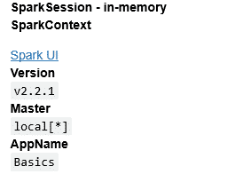

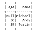
You will first need to get the data from a file (or connect to a large distributed file like HDFS, we’ll talk about this later once we move to larger datasets on AWS EC2).

# We'll discuss how to read other options later.
# This dataset is from Spark's examples

# Might be a little slow locally
df = spark.read.json('people.json')

Showing the data

# Note how data is missing!
df.show()

df.printSchema()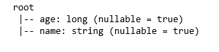

df.columns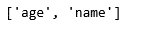

df.describe()

df.describe().show()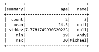

Some data types make it easier to infer schema (like tabular formats such as csv which we will show later).

However you often have to set the schema yourself if you aren’t dealing with a .read method that doesn’t have inferSchema() built-in.

Spark has all the tools you need for this, it just requires a very specific structure:

from pyspark.sql.types import StructField,StringType,IntegerType,StructType

Next we need to create the list of Structure fields

:param name: string, name of the field.
:param dataType: :class:DataType of the field.
:param nullable: boolean, whether the field can be null (None) or not

data_schema = [StructField("age", IntegerType(), True),StructField("name", StringType(), True)]

final_struc = StructType(fields=data_schema)
df = spark.read.json('people.json', schema=final_struc)

df.printSchema()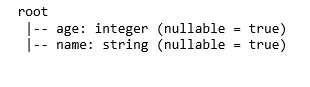

Grabbing the data

df['age']

type(df['age'])

df.select('age')

type(df.select('age'))

df.select('age').show()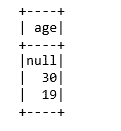

# Returns list of Row objects
df.head(2)

Multiple Columns:

df.select(['age','name'])

df.select(['age','name']).show()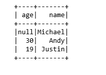

Creating new columns

# Adding a new column with a simple copy
df.withColumn('newage',df['age']).show()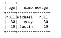

df.show()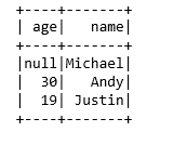

# Simple Rename
df.withColumnRenamed('age','supernewage').show()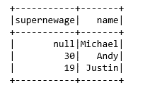

More complicated operations to create new columns

df.withColumn('doubleage',df['age']*2).show()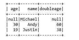

df.withColumn('add_one_age',df['age']+1).show()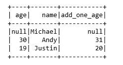

df.withColumn('half_age',df['age']/2).show()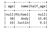

df.withColumn('half_age',df['age']/2)

Using SQL

To use SQL queries directly with the dataframe, you will need to register it to a temporary view:

# Register the DataFrame as a SQL temporary view
df.createOrReplaceTempView("people")

sql_results = spark.sql("SELECT * FROM people")

sql_results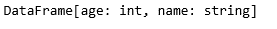

sql_results.show()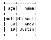

spark.sql("SELECT * FROM people WHERE age=30").show()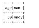

# DataFrame approach
df.filter(df.age == 30).show()

This covers the basics of Dataframes.

Happy Learning!