Introduction to Spectral Clustering

In recent years, spectral clustering has become one of the most popular modern clustering algorithms. It is simple to implement, can be solved efficiently by standard linear algebra software, and very often outperforms traditional clustering algorithms such as the k-means algorithm. On the first glance spectral clustering appears slightly mysterious, and it is not obvious to see why it works at all and what it really does.

Contributed by: Srinivas
LinkedIn Profile: https://www.linkedin.com/in/srinivas-thanniru-a6776b186

What is spectral clustering?

Clustering is one of the most widely used techniques for exploratory data analysis, with applications ranging from statistics, computer science, biology to social sciences or psychology. People attempt to get a first impression on their data by trying to identify groups of “similar behavior” in their data.

Spectral clustering is an EDA technique that reduces complex multidimensional datasets into clusters of similar data in rarer dimensions. The main outline is to cluster the all spectrum of unorganized data points into multiple groups based upon their uniqueness “Spectral clustering is one of the most popular forms of multivariate statistical analysis” ‘Spectral Clustering uses the connectivity approach to clustering’, wherein communities of nodes (i.e. data points) that are connected or immediately next to each other are identified in a graph. The nodes are then mapped to a low-dimensional space that can be easily segregated to form clusters. Spectral Clustering uses information from the eigenvalues (spectrum) of special matrices (i.e. Affinity Matrix, Degree Matrix and Laplacian Matrix) derived from the graph or the data set.

Spectral clustering methods are attractive, easy to implement, reasonably fast especially for sparse data sets up to several thousand. Spectral clustering treats the data clustering as a graph partitioning problem without making any assumption on the form of the data clusters.

Difference between Spectral Clustering and Conventional Clustering Techniques

Spectral clustering is flexible and allows us to cluster non-graphical data as well. It makes no assumptions about the form of the clusters. Clustering techniques, like K-Means, assume that the points assigned to a cluster are spherical about the cluster centre. This is a strong assumption and may not always be relevant. In such cases, Spectral Clustering helps create more accurate clusters. It can correctly cluster observations that actually belong to the same cluster, but are farther off than observations in other clusters, due to dimension reduction.

The data points in Spectral Clustering should be connected, but may not necessarily have convex boundaries, as opposed to the conventional clustering techniques, where clustering is based on the compactness of data points. Although, it is computationally expensive for large datasets, since eigenvalues and eigenvectors need to be computed and clustering is performed on these vectors. Also,for large datasets, the complexity increases and accuracy decreases significantly.

Similarity graphs

Given a set of data points x1,…xn and some notion of similarity sij ≥ 0 between all pairs of data points xi and xj , the intuitive goal of clustering is to divide the data points into several groups such that points in the same group are similar and points in different groups are dissimilar to each other. If we do not have more information than similarities between data points, a nice way of representing the data is in form of the similarity graph G = (V,E). Each vertex vi in this graph represents a data point xi. Two vertices are connected if the similarity sij between the corresponding data points xi and xj is positive or larger than a certain threshold, and the edge is weighted by sij . The problem of clustering can now be reformulated using the similarity graph: we want to find a partition of the graph such that the edges between different groups have very low weights (which means that points in different clusters are dissimilar from each other) and the edges within a group have high weights (which means that points within the same cluster are similar to each other).

To be able to formalize this intuition we first want to introduce some basic graph notation and definitions.

Graph Notations and Definitions

Simple graph: An undirected and unweighted graph containing no loops or multiple edges.

Directed graph: A graph G(V,E) with a set V of vertices and a set E of ordered pairs of vertices, called arcs, directed edges or arrows. If (u,v) ∈ E then we say that u points towards v. The opposite of a directed graph is an undirected graph.

Oriented graph: A directed graph without symmetric pairs of directed edges.

Complete graph: A simple graph in which every pair of distinct vertices is connected by a unique edge.

Tournament: A complete oriented graph

Square of a graph: The square of a directed graph G = (V,E) is the graph G2 = (V,E2) such that (u,w) ∈ E2 if and only if (u,v),(v,w) ∈ E.

Order of a graph: The order of a graph G = (V,E) is the total number of vertices of G, i.e. |V|.

In-degree of a vertex: The number of edges coming into a vertex in a directed graph; also spelt indegree.

Regular graph: A simple graph in which the out-degree of every vertex is equal; also called out-regular graph. In an almost (out-)regular graph, no two out-degrees differ by more than one.

Out-degree of a vertex: The number of edges going out of a vertex in a directed graph; also spelt outdegree.

Tree: A graph in which any two vertices are connected by exactly one simple path. In other words, any connected graph without cycles is a tree.

Leaf: A vertex u ∈ V such that the sum of the out-degree and the in-degree of u is exactly 1.

Forest: A disjoint union of trees.

Oriented cycle: A cycle of edges that are all directed in the same direction; also called directed cycle.

Different Similarity Graphs

There are several popular constructions to transform a given set x1,…,xn of data points with pairwise similarities sij or pairwise distances dij into a graph. When constructing similarity graphs the goal is to model the local neighborhood relationships between the data points.

The ε-neighborhood graph: Here we connect all points whose pairwise distances are smaller than ε. As the distances between all connected points are roughly of the same scale (at most ε), weighting the edges would not incorporate more information about the data to the graph. Hence, the ε-neighborhood graph is usually considered as an unweighted graph.

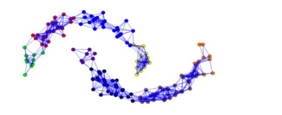
In the Figure below the points within a distance less than ε=0.28 are joined by an edge. It shows that the middle points on each moon are strongly connected, while the points in the extremes less so. In general, it is difficult to define a parameter ε that is robust, especially when the points are distributed with different distances among them depending on the space. If we choose a good parameter ε, we obtain well-defined clusters at the output of the algorithm. As the Figure illustrates the data is grouped into eight clusters represented by different colors.

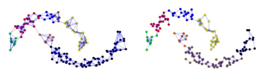
k-nearest neighbor graphs: Here the goal is to connect vertex vi with vertex vj if vj is among the k-nearest neighbors of vi. However, this definition leads to a directed graph, as the neighborhood relationship is not symmetric. There are two ways of making this graph undirected. The first way is to simply ignore the directions of the edges, that is we connect vi and vj with an undirected edge if vi is among the k-nearest neighbors of vj or if vj is among the k-nearest neighbors of vi. The resulting graph is what is usually called the k-nearest neighbor graph. The second choice is to connect vertices vi and vj if both vi is among the k-nearest neighbors of vj and vj is among the k-nearest neighbors of vi. The resulting graph is called the mutual k-nearest neighbor graph. In both cases, after connecting the appropriate vertices we weight the edges by the similarity of their endpoints.

The fully connected graph: Here we simply connect all points with positive similarity with each other, and we weight all edges by sij . As the graph should represent the local neighborhood relationships, this construction is only useful if the similarity function itself models local neighborhoods. An example for such a similarity function is the Gaussian similarity function s(xi, xj ) = exp(−(xi − xj(2/(2σ2)), where the parameter σ controls the width of the neighborhoods. This parameter plays a similar role as the parameter ε in case of the ε-neighborhood graph.

Spectral Clustering Matrix Representation

Adjacency and Affinity Matrix (A)

The graph (or set of data points) can be represented as an Adjacency Matrix, where the row and column indices represent the nodes, and the entries represent the absence or presence of an edge between the nodes (i.e. if the entry in row 0 and column 1 is 1, it would indicate that node 0 is connected to node 1).

An Affinity Matrix is like an Adjacency Matrix, except the value for a pair of points expresses how similar those points are to each other. If pairs of points are very dissimilar then the affinity should be 0. If the points are identical, then the affinity might be 1. In this way, the affinity acts like the weights for the edges on our graph.

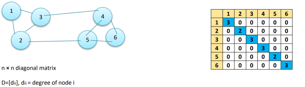
Degree Matrix (D)

A Degree Matrix is a diagonal matrix, where the degree of a node (i.e. values) of the diagonal is given by the number of edges connected to it. We can also obtain the degree of the nodes by taking the sum of each row in the adjacency matrix.

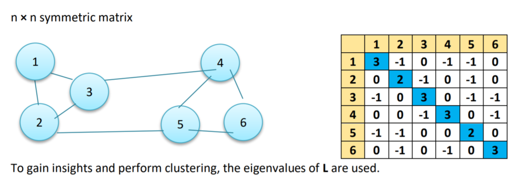
Laplacian Matrix (L)

This is another representation of the graph/data points, which attributes to the beautiful properties leveraged by Spectral Clustering. One such representation is obtained by subtracting the Adjacency Matrix from the Degree Matrix (i.e. L = D – A).

Spectral Gap: The first non-zero eigenvalue is called the Spectral Gap. The Spectral Gap gives us some notion of the density of the graph.

Fiedler Value: The second eigenvalue is called the Fiedler Value, and the corresponding vector is the Fiedler vector. Each value in the Fiedler vector gives us information as to which side of the decision boundary a particular node belongs to.
Using L, we find the first large gap between eigenvalues which generally indicates that the number of eigenvalues before this gap is equal to the number of clusters.

Graph Laplacians

The unnormalized graph Laplacian L = D – W

The normalized graph Laplacians- There are two matrices which are called normalized graph Laplacians in the literature. Both matrices are closely related to each other and are defined as Lsym := D−1/2LD−1/2 = I − D−1/2W D−1/2
Lrw := D−1L = I − D−1W.

We denote the first matrix by Lsym as it is a symmetric matrix, and the second one by Lrw as it is closely related to a random walk Eigenvectors and Eigenvalues.

We often using these terms Eigenvectors and Eigenvalues in this article, to understand more about them, For a matrix A, if there exists a vector x which isn’t all 0’s and a scalar λ such that Ax = λx, then x is said to be an eigenvector of A with corresponding eigenvalue λ.

We can think of the matrix A as a function which maps vectors to new vectors. Most vectors will end up somewhere completely different when A is applied to them, but eigenvectors only change in magnitude.

If we drew a line through the origin and the eigenvector, then after the mapping, the eigenvector would still land on the line. The amount which the vector is scaled along the line depends on λ.

Eigenvectors are an important part of linear algebra, because they help describe the dynamics of systems represented by matrices. There are numerous applications which utilize eigenvectors, and we’ll use them directly here to perform spectral clustering.

“Eigenvalues are non-negative real numbers and Eigenvectors are real and orthogonal”

Spectral Clustering Algorithms

We assume that our data consists of n “points” x1,…,xn which can be arbitrary objects. We measure their pairwise similarities sij = s(xi, xj ) by some similarity function which is symmetric and non-negative, and we denote the corresponding similarity matrix by S = (sij )i,j=1…n.

Unnormalized spectral clustering

Input: Similarity matrix S ∈ n×n, number k of clusters to construct.

Construct a similarity graph by one of the ways described in Section 2. Let W be its weighted adjacency matrix.
Compute the unnormalized Laplacian L.
Compute the first k eigenvectors u1,…,uk of L.
Let U ∈ n×k be the matrix containing the vectors u1,…,uk as columns.
For i = 1,…,n, let yi ∈ k be the vector corresponding to the i-th row of U.
Cluster the points (yi)i=1,…,n in k with the k-means algorithm into clusters C1,…,Ck.
Output: Clusters A1,…,Ak with Ai = {j| yj ∈ Ci}.

Normalized spectral clustering according to Shi and Malik (2000)

Input: Similarity matrix S ∈ n×n, number k of clusters to construct.
Construct a similarity graph by one of the ways described in Section 2. Let W be its weighted adjacency matrix.
Compute the unnormalized Laplacian L.
Compute the first k generalized eigenvectors u1,…,uk of the generalized eigenproblem Lu = λDu.
Let U ∈ n×k be the matrix containing the vectors u1,…,uk as columns.
For i = 1,…,n, let yi ∈ k be the vector corresponding to the i-th row of U.
Cluster the points (yi)i=1,…,n in k with the k-means algorithm into clusters C1,…,Ck.
Output: Clusters A1,…,Ak with Ai = {j| yj ∈ Ci}.
Normalized spectral clustering according to Ng, Jordan, and Weiss (2002)
Input: Similarity matrix S ∈ n×n, number k of clusters to construct.

Construct a similarity graph by one of the ways described in Section 2. Let W be its weighted adjacency matrix.
Compute the normalized Laplacian Lsym.
Compute the first k eigenvectors u1,…,uk of Lsym.
Let U ∈ n×k be the matrix containing the vectors u1,…,uk as columns.
Form the matrix T ∈ n×k from U by normalizing the rows to norm 1, that is set tij = uij/( ” k u2 ik)1/2.
For i = 1,…,n, let yi ∈ k be the vector corresponding to the i-th row of T.
Cluster the points (yi)i=1,…,n with the k-means algorithm into clusters C1,…,Ck.
Output: Clusters A1,…,Ak with Ai = {j| yj ∈
All three algorithms stated above look rather similar, apart from the fact that they use three different graph Laplacians. In all three algorithms, the main trick is to change the representation of the abstract data points xi to points yi ∈ k. It is due to the properties of the graph Laplacians that this change of representation is useful.

Graph cut

We wish to partition the graph G(V, E) into two disjoint sets of connected vertices A and B: by simply removing edges connecting two parts.

• We define the degree di of a vertex i as the sum of edges weights incident to it: The degree matrix of the graph G denoted by will be a diagonal matrix having the elements on its diagonal and the off-diagonal elements having value 0.

 Given two disjoint clusters (subgraphs) A and B of the graph G, we define the following three terms:

The sum of weight connections between two clusters:

The sum of weight connections within cluster A:

The total weights of edges originating from cluster A

In graph theory, there are different objective functions:

✓ Minimum cut method

✓ Ratio cut method

✓ Normalized cut method

✓ MinMaxCut cut method