- Gaussian Mixture Model: Introduction
- What is a Gaussian Mixture Model?
- Why do we use the Variance-Covariance Matrix?
- K-Means VS Gaussian Mixture Model
- Usage of EM Algorithm
- Applications
Contributed by: Gautam Solanki
Introduction
Gaussian Mixture Model or Mixture of Gaussian as it is sometimes called, is not so much a model as it is a probability distribution. It is a universally used model for generative unsupervised learning or clustering. It is also called Expectation-Maximization Clustering or EM Clustering and is based on the optimization strategy. Gaussian Mixture models are used for representing Normally Distributed subpopulations within an overall population. The advantage of Mixture models is that they do not require which subpopulation a data point belongs to. It allows the model to learn the subpopulations automatically. This constitutes a form of unsupervised learning.
A Gaussian is a type of distribution, and it is a popular and mathematically convenient type of distribution. A distribution is a listing of outcomes of an experiment and the probability associated with each outcome. Let’s take an example to understand. We have a data table that lists a set of cyclist’s speeds.
| Speed (Km/h) | Frequency |
| 1 | 4 |
| 2 | 9 |
| 3 | 6 |
| 4 | 7 |
| 5 | 3 |
| 6 | 2 |
Here, we can see that a cyclist reaches the speed of 1 Km/h four times, 2Km/h nine times, 3 Km/h and so on. We can notice how this follows, the frequency goes up and then it goes down. It looks like it follows a kind of bell curve the frequencies go up as the speed goes up and then it has a peak value and then it goes down again, and we can represent this using a bell curve otherwise known as a Gaussian distribution.
A Gaussian distribution is a type of distribution where half of the data falls on the left of it, and the other half of the data falls on the right of it. It's an even distribution, and one can notice just by the thought of it intuitively that it is very mathematically convenient.
Also Read: A complete understanding of LASSO Regression
So, what do we need to define a Gaussian or Normal Distribution? We need a mean which is the average of all the data points. That is going to define the centre of the curve, and the standard deviation which describes how to spread out the data is. Gaussian distribution would be a great distribution to model the data in those cases where the data reaches a peak and then decreases. Similarly, in Multi Gaussian Distribution, we will have multiple peaks with multiple means and multiple standard deviations.
The formula for Gaussian distribution using the mean and the standard deviation called the Probability Density Function:
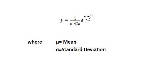
For a given point X, we can compute the associated Y values. Y values are the probabilities for those X values. So, for any X value, we can calculate the probability of that X value being a part of the curve or being a part of the dataset.
This is a function of a continuous random variable whose integral across an interval gives the probability that the value of the variable lies within the same interval.
What is a Gaussian Mixture Model?
Sometimes our data has multiple distributions or it has multiple peaks. It does not always have one peak, and one can notice that by looking at the data set. It will look like there are multiple peaks happening here and there. There are two peak points and the data seems to be going up and down twice or maybe three times or four times. But if there are Multiple Gaussian distributions that can represent this data, then we can build what we called a Gaussian Mixture Model.
In other words we can say that, if we have three Gaussian Distribution as GD1, GD2, GD3 having mean as µ1, µ2,µ3 and variance 1,2,3 than for a given set of data points GMM will identify the probability of each data point belonging to each of these distributions.
It is a probability distribution that consists of multiple probability distributions and has Multiple Gaussians.
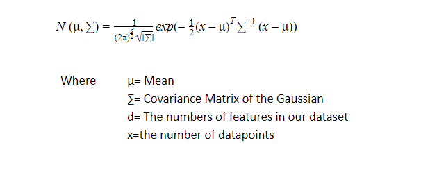
The probability distribution function of d-dimensions Gaussian Distribution is defined as:
Why do we use the Variance-Covariance Matrix?
The Covariance is a measure of how changes in one variable are associated with changes in a second variable. It's not about the independence of variation of two variables but how they change depending on each other. The variance-covariance matrix is a measure of how these variables are related to each other, and in that way it's very similar to the standard deviation except when we have more dimension, the covariance matrix against the standard deviation gives us a better more accurate result.
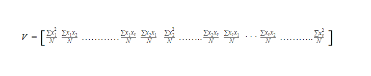
Where, V= c x c variance-covariance matrix
N = the number of scores in each of the c datasets
xi= is a deviation score from the ith dataset
xi2/N= is the variance of element from the ith dataset
xixj/N= is the covariance for the elements from the ithand jth datasets
and the probability given in a mixture of K Gaussian where K is a number of distributions:
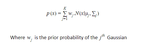

Once we multiply the probability distribution function of d-dimension by W, the prior probability of each of our gaussians, it will give us the probability value X for a given X data point. If we were to plot multiple Gaussian distributions, it would be multiple bell curves. What we really want is a single continuous curve that consists of multiple bell curves. Once we have that huge continuous curve then for the given data points, it can tell us the probability that it is going to belong to a specific class.
Now, we would like to find the maximum likelihood estimate of X (the data point we want to predict the probability) i.e. we want to maximize the likelihood that X belongs to a particular class or we want to find a class that this data point X is most likely to be part of.
It is very similar to the k-means algorithm. It uses the same optimization strategy which is the expectation maximization algorithm.
K-Means VS Gaussian Mixture Model
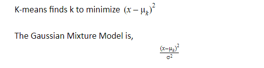
The reason that standard deviation is added into this because in the denominator the 2 takes variation into consideration when it calculates its measurement but K means only calculates conventional Euclidean distance. i.e K-means calculates distance and GM calculates weights.
This means that the k-means algorithm gives you a hard assignment: it either says this is going to be this data point is a part of this class or it's a part of this class. In a lot of cases we just want that hard assignment but in a lot of cases it's better to have a soft assignment. Sometimes we want the maximum probability like: This is going to be 70% likely that it's a part of this class but we also want the probability that it's going to be a part of other classes. It is a list of probability values that it could be a part of multiple distributions, it could be in the middle, it could be 60% likely this class and 40% likely of this class. That's why we incorporate the standard deviation.
Expectation Maximization Algorithm: EM can be used for variables that are not directly observable and deduce from the value of other observed variables. It can be used with unlabeled data for its classification. It is one of the popular approaches to maximize the likelihood.
Basic Ideas of EM -Algorithm: Given a set of incomplete data and set of starting parameters.
E-Step: Using the given data and the current value of parameters, estimate the value of hidden data.
M-Step: After the E-step, it is used to maximize the hidden variable and joint distribution of the data.
Usage of EM Algorithm
- Can be used to fill missing data.
- To find the values of latent variables.
The disadvantage of EM algorithm is that it has slow convergence and it converges up to local optima only.
Comparing to Gradient descent
Gradient descent compute the derivative which tells us the direction in which the data wants to move in or in what direction should we move the parameter’s data of your model such that the function of our model is optimized to fit our data but what if we can't compute a gradient of a variable. i.e. we can't compute a derivative of a random variable. The Gaussian mixture model has a random variable. It is a stochastic model i.e. it is non-deterministic. We can't compute the derivative of a random variable that's why we cannot use gradient descent.
Applications
- GMM is widely used in the field of signal processing.
- GMM provides good results in language Identification.
- Customer Churn is another example.
- GMM founds its use case in Anomaly Detection.
- GMM is also used to track the object in a video frame.
- GMM can also be used to classify songs based on genres.
This brings us to the end of the blog on Gaussian Mixture Model. We hope you enjoyed it. If you wish to learn more such concepts, upskill with Great Learning Academy's free online courses.