As you manage the inventory, organize the customer information, or bring together some financial reports, you will continue having a powerful instrument that allows for easy handling of copious data in the form of Excel.
One of EXCEL's most popular and multi-purpose functions is VLOOKUP, which is short for “vertical lookup”. If you have ever needed to look for particular information in a giant spreadsheet, for example, the price of a product with an ID or an employee’s name, based on their ID number, VLOOKUP can save you from hours of manual search.
In this tutorial, we will help you use the VLOOKUP function in Excel, its syntax, and common errors to avoid.
Learn Excel for powerful data analysis and enhance your skills for better decision-making.
What is VLOOKUP?
The VLOOKUP function in Microsoft Excel is an effective tool that searches for specific values in the table's first column and produces related data in another column under the same row.
Referred to as “Vertical Lookup”, it’s perfect for obtaining data like the employee’s name by ID or the product’s price by the code, being necessary for analyzing and reporting data, and managing massive datasets seamlessly.
Understanding the VLOOKUP Syntax
The basic syntax of the VLOOKUP function is:
=VLOOKUP(lookup_value, table_array, col_index_num, [range_lookup])
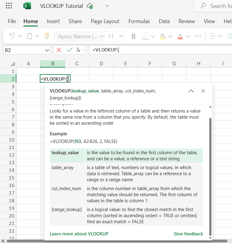
Let's break down each component:
- lookup_value (required): This is the value you want to search for in the first column of your data range. It can be a specific value or a cell reference.
- table_array (required): This is the cell range containing the data. The first column of this range should include the lookup value.
- col_index_num (required): This is the column number in the table_array to retrieve the value. The first column is 1, the second is 2, and so on.
- [range_lookup](optional): This argument specifies whether you want an exact match or an approximate match:
- TRUE or omitted: Finds the closest match less than or equal to the lookup_value. The first column must be sorted in ascending order.
- FALSE: Finds an exact match. If none is found, the function returns a #N/A error.
Example
Suppose you have the following data:
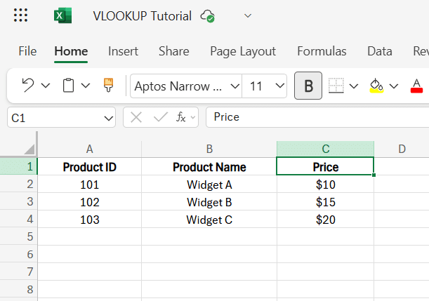
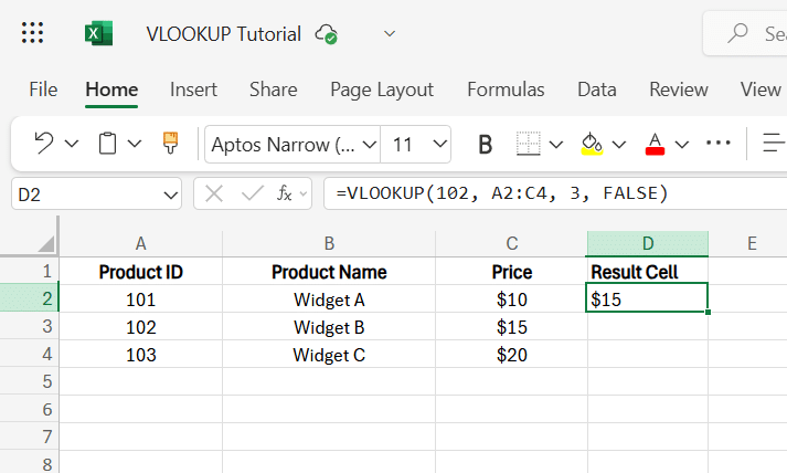
To find the price of the product with ID 102, you would use:
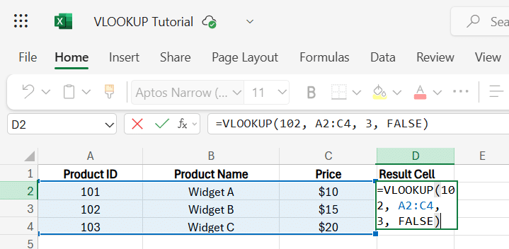
This formula looks for 102 in the first column of the range A2:C4 and returns the value from the third column, $15.
Important Notes
- Data Arrangement: The lookup_value has to be in the first column of the table_array. VLOOKUP can only search to the right of the lookup_value column.
- Exact vs. Approximate Match: Use FALSE for an exact match to reduce unexpected results. If TRUE or null, guarantee that the first column of the table_array is sorted in ascending order.
- Case Sensitivity: VLOOKUP is insensitive to cases; it regards upper and lower case letters as the same.
Step-by-Step Guide: How to Use VLOOKUP in Excel (With Example)
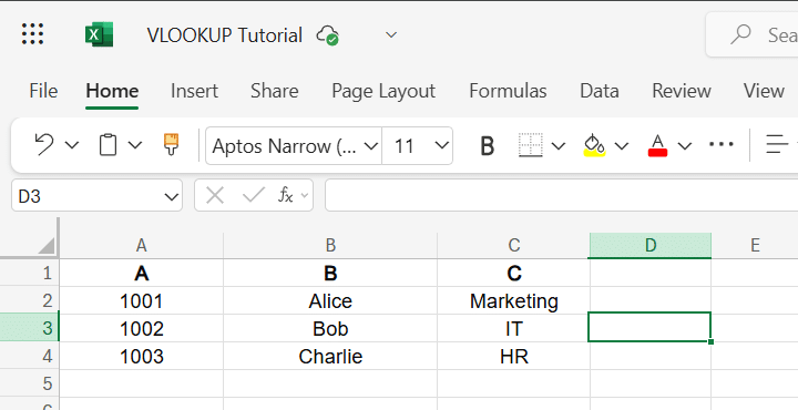
Step 1: Organize Your Data
Before using VLOOKUP, your data must be arranged correctly. The column containing the lookup values must be your table array's first (leftmost) column.
Example Table:
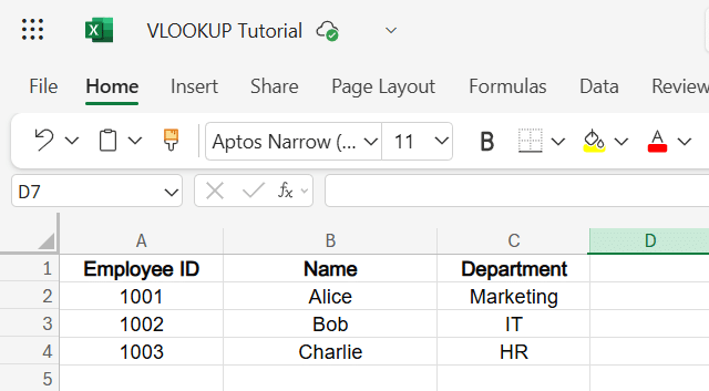
In this example, we’ll look up an Employee ID and return the corresponding Department.
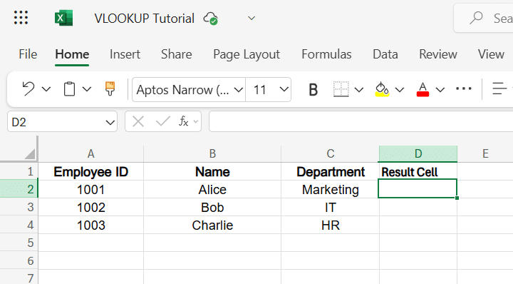
Step 2: Select the Cell for the Result
Click on the cell where you want the VLOOKUP result to appear.
Let’s say you want to display the department of employee ID 1002 in cell D2.
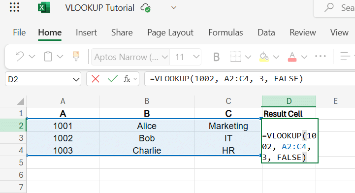
Step 3: Enter the VLOOKUP Formula
Begin typing the VLOOKUP function with its required arguments:
=VLOOKUP(1002, A2:C4, 3, FALSE)
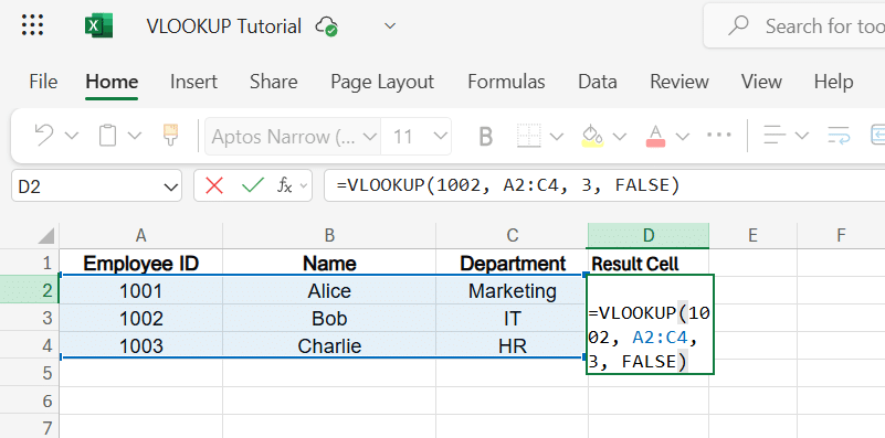
Let’s break this down:
- 1002 → This is the lookup_value, the value you want to find in the first column.
- A2:C4 → This is the table_array, the range containing both the lookup and return values.
- 3 → This is the col_index_num, which tells Excel to return the value from the third column (Department).
- FALSE → This tells Excel to find an exact match.
Step 4: Specify Exact or Approximate Match

The fourth argument in VLOOKUP is optional, but critical:
- Use FALSE for exact match (most common in business tasks like employee IDs, product codes, etc.).
- Use TRUE (or omit the argument) for the approximate match (applicable in scenarios like grade thresholds or tax brackets).
Important: If using TRUE, the first column in the table must be sorted in ascending order for reliable results.
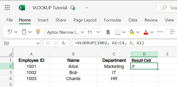
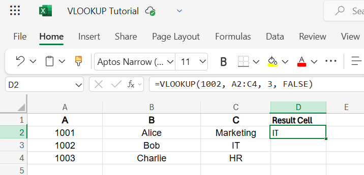
Step 5: Press Enter and Review the Result
Once you've entered the formula, press Enter.
If the value exists, Excel will return the matching value from the specified column, in our case, “IT” for Employee ID 1002.
If there’s no match, you’ll see:
- #N/A → The lookup value wasn’t found in the first column.
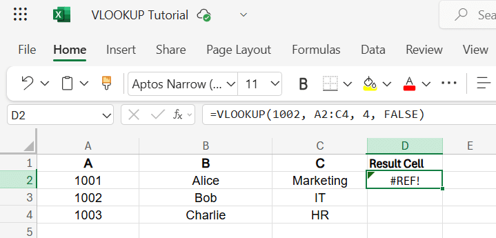
- #REF! → The col_index_num is greater than the number of columns in the table_array.
- #VALUE! → There might be a syntax error or incorrect argument type.
Master functions like VLOOKUP, Pivot Tables, and more with the Excel Training (Beginner to Advanced) program by Great Learning today.
Common VLOOKUP Mistakes and How to Fix Them
1. Incorrect Column Index Number
Scenario: You want to find the department of Employee ID 1002.
Formula Used (Mistake):
=VLOOKUP(1002, A2:C4, 4, FALSE)
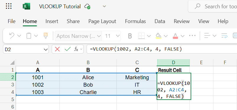
Issue: Column index 4 doesn’t exist in the range A2:C4.
Result: #REF! Error.
Fix:
=VLOOKUP(1002, A2:C4, 3, FALSE)
Now it returns: "IT"
2. Forgetting Absolute References
Scenario: You’re applying VLOOKUP across multiple rows to pull departments for multiple employee IDs listed in Column E.
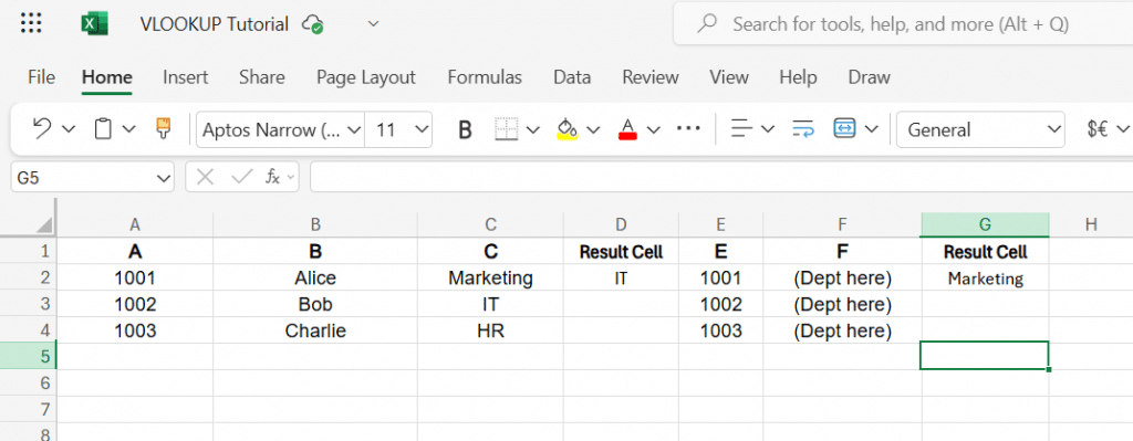
Formula Used (Mistake in F2):
=VLOOKUP(E2, A2:C4, 3, FALSE)
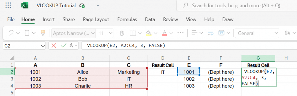
Issue: When you drag the formula down, A2:C4 might change to A3:C5, resulting in wrong or missing values.
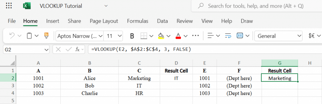
Fix:
=VLOOKUP(E2, $A$2:$C$4, 3, FALSE)
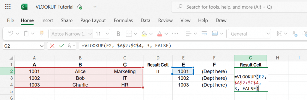
Use $ to lock the lookup range; the result will be Marketing.
3. Not Sorting with Approximate Match
Scenario: Grading students based on score thresholds:
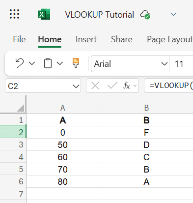
Lookup Value (Score): 65
Formula (Correct with Sorted Data):
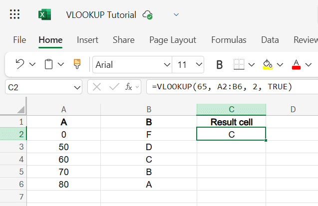
=VLOOKUP(65, A2:B6, 2, TRUE)
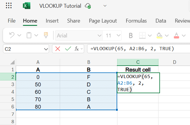
Result: "C" (correct)
Mistake: If column A is not sorted, VLOOKUP might return incorrect grades.
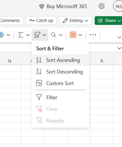
Fix:
Always sort column A in ascending order if using TRUE.
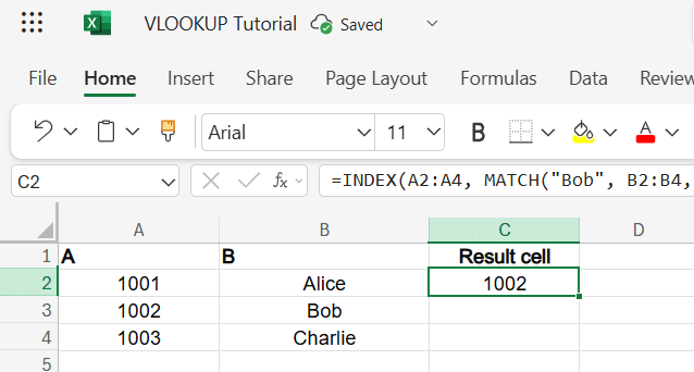
4. Lookup Column Is Not First
Scenario: You want to find the Employee ID based on the employee's name.

Formula (Incorrect):
=VLOOKUP("Bob", A2:B4, 1, FALSE)
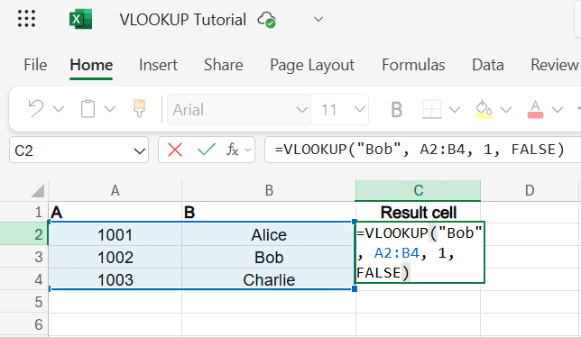
Issue: VLOOKUP only looks to the right of the lookup column. It fails since “Bob” is in column B (the second column).
Fix (Rearrange or use INDEX+MATCH):
=INDEX(A2:A4, MATCH("Bob", B2:B4, 0))

Result: 1002
Conclusion
Proficiency with the VLOOKUP function in Excel can significantly boost your capacity to manage data, automate reports, perform data analysis of business trends, or make informed decisions. However, this is just the beginning of an Excel, all. If you wish to extend your skills to a higher level, then you must consider going for Great Learning’s course in Data Science and Business Analytics. It intends to train professionals on the real-world data tools such as Excel, SQL, Python, etc, to make you feel confident to solve complex business problems.