Introduction to Excel
Over the years, MS Excel has become more of a skill than an application. Although it is very underrated, the importance it has in the daily life of a working professional is very significant. Listed are some of the most important Excel interview questions you should learn answers to.
This is a beginner to advanced course, covering Data Visualization, Pivot Tables, Conditional Formatting, Data Cleaning, Cell Referencing, If-Else Logic, Budgeting Techniques, Business Intelligence, and ChatGPT in Excel.
Learn Excel the smart way! Our course teaches you all the essential tools and techniques to master spreadsheets, from formulas to charts, and improve your workflow in every task you do.
Basic Excel interview questions
1. What is MS Excel?
Microsoft Excel, also commonly denoted as MS Excel, is a widely used application of Microsoft Office. It is an electronic spreadsheet that enables users to store, organize, and analyze data in the format of a table. Users can work on MS Excel with Microsoft Windows and Mac OS operating systems on their computers. It is also available as a mobile application on Android and iOS platforms. It is commercially used by businesses as a part of the MS Office Suite.
2. How to remove duplicates in Excel?
To remove duplicates in Excel, follow these steps –
- Select the range of cells that you want to remove.
- Click Data.
- Under the columns in the Data Group, click Remove Duplicates.
- Check or uncheck the columns where you want to remove duplicates.
- Click OK.
- A message will appear showing how many duplicates were removed.
3. How to calculate percentages in Excel?
Follow these steps to calculate a percentage in an Excel spreadsheet–
- Select the desired cell to display the percentage.
- Start by typing an equal (‘=’) sign.
- Apply the basic formula for percentage which is = part/total.
- Type A1/A2 and hit Enter.
- Click Home and select the percent (% ) symbol from the numbers group.
- The result will be displayed as decimal fractions.
4. How to freeze rows in Excel?
- Select the rows you want to freeze.
- Click View in the main menu.
- Go to the Ribbon, click ‘Freeze Panes’, and then again click ‘Freeze Panes.’
5. How to merge cells in Excel?
- Select the cell where you want to merge the combined data.
- Click on the first cell and select the range you want to merge.
- Click Home.
- Select “Merge & Center” from the menu.
6. How to convert a PDF to Excel?
- Open the PDF document you want to convert in XLSX format in Acrobat DC.
- Go to the right pane and click on the “Export PDF” option.
- Choose spreadsheet as the Export format.
- Select “Microsoft Excel Workbook.”
- Now click “Export.”
- Download the converted file or share it.
7. How to enable macros in Excel?
- Click the file tab and then click “Options.”
- A dialog box will appear. In the “Excel Options” dialog box, click on the “Trust Center” and then “Trust Center Settings.”
- Go to the “Macro Settings” and select “enable all macros.”
- Click OK to apply the macro settings.
8. How to convert Excel to PDF?
- Select the MS Excel file you want to convert to PDF.
- Click on the File menu on the top-left corner.
- It will open an Export Panel. Click “Export” from the menu.
- Look for “Create PDF/XPS document.”
- On the “Options” tab, you can adjust the settings accordingly.
- Choose the PDF options to save the spreadsheet as a PDF.
- Under the tab “Publish What,” choose Active Sheet(s) if you wish to save the entire worksheet as PDF or select “Selection” if you wish to save the selected area as PDF.
- Click OK to continue.
- Choose the folder location to save the new file.
- Name the file and hit “publish.” The new file will be saved as a PDF file.
9. How to change date format in excel?
- First, select the cells containing the date.
- Right-click on the mouse or keypad and select “Format” cells.
- Go to the “Number” tab and select “Custom.”
- Then type the date format you want in the Type box.
- Click OK to continue.
- It will format the selected dates.
10. How to add a drop-down in Excel?
Here is how to create a drop-down list in Excel –
- Select the cells you want to contain in the drop-down list.
- Go to the ribbon and click “Data,” then “Data Validation.”
- In the dialog box, select “Allow to List.”
- Click on Source and type the numbers or text that you want in your drop-down lists.
- Click OK to continue.
- Note that commas should separate the numbers and texts.
Master the fundamentals of spreadsheets with the Excel for Beginners course. Learn essential Excel functions, formulas, and data tools, all for free.
Excel for Beginners Free Course
Learn essential Excel skills for data analysis, including functions, formulas, and data visualization techniques. Master cell referencing, sorting, and creating charts and presentations.
11. How to use VLOOKUP in Excel?
- Click the cell where you want the VLOOKUP formula to be calculated.
- Go to the top of the screen and click “Formulas.”
- Click on “Lookup and Reference” on the ribbon.
- At the bottom of the drop-down menu, look for VLOOKUP.
- Select the cell in which you want to apply the formula.
- A VLOOKUP dialog box will open; specify the data you want to use for search in the “Table_array” box.
- Specify the column number.
- Specify “Range_Lookup” by entering either True or False. If you want an exact match, enter FALSE.
- Click OK to continue.
- Now enter the value for the data you are searching for.
- VLOOKUP will automatically produce the desired result.
Check out this Excel VLOOKUP course to learn VLOOKUP in detail.
12. How to split cells in Excel?
- Select the cell or cells with the data you want to split.
- Click the “Layout” tab.
- Click “Split Cells” in the Merge group tab.
- A dialog will appear. In the Split Cells dialog, enter the number of columns and rows you want.
- Click OK to save changes.
- The cell will be split into fragments.
13. How to multiply in Excel?
The easiest way to multiply in Excel is by using a simple formula for multiplication using the asterisk symbol. It enables users to multiply individual cells and numbers. All you have to do is separate them by commas. To multiply a series, use a colon.
For example, using the formula – “=PRODUCT (A1, A2:A5, B1,12)”, Excel will multiply (A1XA2XA3XA4XA5XB1X12). Here, A2:A5 indicates that it should multiply A2, A3, A4, and A5.
Another way to do multiplication in Excel is using the following steps –
- Type “=” in a cell.
- Click the first cell containing the number you want to multiply.
- Type “*”.
- Now, click the second cell.
- Press Enter. The result of multiplication will appear.
14. How to unprotect an Excel sheet?
- Go to “File.”
- Select Info>Protect>Unprotect Sheet
- You can skip this step and also do the changes from the Review tab. Go to Changes>Unprotect Sheet.
- Enter the password to proceed in case the sheet is password protected.
- Otherwise, click OK to continue.
15. How to subtract in Excel?
- Select the cell where you want the subtraction result to appear.
- Start by typing “=” in the cell.
- Apply the subtraction formula. Enter this syntax – “=MINUS(value1value2) where Value 1 and Value 2 can be numbers, cells, dates, etc.
- Press the Enter key.
- The difference between the values will appear in that cell.
16. How to convert numbers to words in Excel in rupees?
- Select a cell adjacent to the cell you want the currency (Rupees) to be converted into words.
- Enter the formula – NumberstoWords(A1) and press Enter. A1 is the cell containing the currency in Rupees.
- Press Enter to confirm the formula.
17. How to round off in Excel?
You can use the ROUNDUP function to round off in Excel. Here is how –
- Select a blank cell.
- Use the ROUND function by entering the syntax – “=ROUNDUP(number,num_digits).
Where number denotes the number to round up, and num_digits refers to the number of digits to which it should be rounded up.
- Press Return.
Using the button, you can round off in Excel by following these steps –
- Select the cells you want to round off.
- Go to the Home tab, click Increase Decimal or Decrease Decimal.
- Press Enter.
18. How to unhide rows in Excel?
Follow these steps to unhide hidden rows in Excel:
- Navigate to the Home tab.
- Go to the right side of the toolbar and click “Format.”
- Go to the “Visibility” section.
- Hover over “Hide & Unhide.”
- Select “Unhide Rows” from the menu.
- Press Enter.
19. How to find percentages in Excel?
Follow these steps to show a number as a percent in Excel –
- Select the cells you want to format.
- Navigate to the ribbon’s Home tab and locate the Numbers group.
- Click the “Percent style” button.
- You can increase or decrease the percentage as you like.
20. What is VLOOKUP in Excel?
VLOOKUP is an acronym for Vertical Lookup in Excel. It is a function that looks up a certain value in a column, like a name, number, or data, and returns with the corresponding value from a different column in the same row.
For example, using the VLOOKUP function, you can look up the first name and return the salary corresponding to that name. It should be noted that the VLOOKUP function is case-sensitive.
21. How to find duplicates in Excel?
- Select the cells you want to check for duplicates.
- Navigate to Home. Click “Conditional Formatting.”
- Then click Highlight Cells Rules> Duplicate Values.
- Pick the formatting you want to apply to the duplicate values in the box.
- Click OK to continue.
22. How to make a graph in Excel?
- Start by selecting the data for which you want to create a graph.
- Choose from the suitable graph options.
- Highlight the data.
- Click “Insert” and choose your desired graph from “Recommended Charts.”
- Adjust the layout or colors as per your preferences.
- Click Ok to continue.
23. How to compare two columns in Excel?
You can compare two columns in Excel using the simple IF formula. The syntax to be used is =IF(A2=B2,”Match,” Mismatch”)
If the values to be compared are case-sensitive, use the following formula
=IF(EXACT(A2,B2),”Match”,”Mismatch”)
24. How to remove blank rows in Excel?
Delete blank rows in Excel using these steps –
- Navigate to the Home tab.
- Go to the “Editing Group” and click “Find & Select.”
- Click “Go to special.”
- Select the blank rows and click OK.
- Click “Delete.”
- Click “Delete Sheet Rows” and press Enter.
25. How to learn Excel?
You can learn Excel with the help of various online courses, most of which are usually available for free. Once you learn the basics, you can start practicing some of the easiest Maths problems in Excel, creating tables and charts. You can also opt for an advanced online course to learn and earn a Microsoft Excel Specialist certification. ‘
26. How to remove the formula in Excel?
- Select the cells or rows that contain the formula.
- Go to the Home tab and the “Editing Group.”
- Click “Find & Select” and then “Go To.
- Click “Special” and then “Current Array.”
- Press DELETE.
Explore Excel Formulas to boost your spreadsheet skills with essential functions and examples.
27. How to add in Excel?
One of the easiest ways to do addition in Excel is using the feature AutoSum. Here is how to do it –
- Click on an empty cell.
- Go to the “Formula” tab and click “Autosum”>Sum.
- The sum will appear in the result.
28. How to remove space in Excel?
To remove extra spaces in Excel –
- Press Ctrl+Space to select cells in a column.
- Open the “Find & Replace” dialog box using the shortcut Ctrl+H.
- In the “Find What” field, press the spacebar.
- Leave the “Replace with” field empty.
- Click on “Replace all” and press OK. All spaces will be removed.
29. How to calculate age in Excel?
The easiest way to calculate age in MS Excel is using the formula –
“=DATEDIF(birth_date,as_of_date,”y”)”
The result will be the number of complete years.
30. How to calculate the average in Excel?
- Click on the empty cell below the cells containing numbers you want to find the average.
- Navigate to the “Home” tab and go to the “Editing Group.”
- Click the arrow next to the “Autosum.”
- Click Average and press Enter.
31. How to remove the scroll lock in Excel?
- Click on the Settings>Select Ease of Access>Keyboard.
- Use the On-screen keyboard or use the shortcut Windows logo key + Ctrl + O.
- Click the “ScrLk” button.
- Right-click with your mouse or keypad.
- You can click on the status bar to either display or hide the scroll lock.
32. How to compare two Excel sheets?
You can easily compare two Excel sheets using the “view side by side” option. It is recommended while comparing small datasets manually. In the case of a large dataset, it is best to use the formula method.
Using the “View side by side” option –
- Open the files and select the sheets you want to compare.
- Click the “View” tab.
- Click the “View Side By Side” option in the Windows group.
- When you click OK, Excel will arrange both sheets to be viewed horizontally, and you can compare them side by side.
33. How to lock cells in Excel?
Here are the steps to lock cells in Excel for protection and added security –
- Select the cells you want to lock.
- Go to the “home” tab and navigate to the “Alignment” group.
- Click on the arrow, and it will open the “Format Cells” dialog box.
- Go to the “Protection” tab and select the “Loaded” checkbox.
- Click OK to continue.
34. How many rows and columns are in Excel?
There are 1,048,576 rows and 16,384 columns in a Microsoft Excel sheet, along with 1,026 horizontal and vertical page breaks.
35. How to search in Excel?
To search for something in Excel, use these steps –
- Navigate to the “Home” tab and click “Find & Select.”
- Go to Find>Find What, and a box will appear.
- Type the text or numbers you want to search or find.
- Click “Find Next,” and it will run your search.
- The search will return the results.
36. What is the shortcut to change small letters to capital letters in Excel?
You can use the shortcut key Shift + F3 to change the text from lowercase to uppercase and vice versa.
37. How to filter in Excel?
- Select the desired cell.
- Go to “Data” and click “Filter” in the Sort & Filter group.
- Select the column header. It will display a list with filter choices.
- Select between “Text Filters” or “Number Filters” in the list.
- Select a Comparison and enter the filter criteria.
- Click Ok to see changes.
38. How to use the pivot table in Excel?
- Click the desired cell.
- Click Insert > PivotTable.
- The “Create PivotTable” dialog box will appear.
- Select a table or range as per your requirement.
- Select either the New worksheet or the Existing worksheet under the “Choose where you want the PivotTable report to be placed” option.
- After selecting the location for PivotTable to appear, click OK to continue.
39. How to sort in Excel?
If you want to sort by column or row in the Excel sheet, follow these steps –
- Select the desired cell in the data range.
- Navigate to the “Data” tab.
- Go to the “Sort & Filter” group and click “Sort.”
- The “Sort” dialog box will appear. Go to “Column,” and under it, select the column you want to sort.
- Select the type of sort under “Sort On.”
- Select how you want to order under the option “Under Order.”
- Click Ok to see the changes.
40. What is the extension of the saved file in MS Excel?
Microsoft Excel saved file has a .xls extension. The XLS-based extension has been used as the default format for Microsoft Excel 1997-2003. Files saved in the .xlsx extension are associated with Microsoft Excel 2007-10.
41. How to unprotect an Excel sheet without a password?
- Navigate to the worksheet tab at the bottom of your screen.
- Right-click on it and select “Unprotect Sheet” in the Context menu.
- Click the Unprotect sheet from the drop-down menu.
- If the sheet is password-protected, Excel will ask you to enter the password.
- Type the password and click OK to continue.
42. How to open the XML file in Excel?
- Open MS Excel.
- Click File and then click Open.
- Browse for the XML file and click on Open file.
- A pop-up box with three options will open. Select the radio button with As an XML table option.
- Click Ok to continue and open the XML file in Excel.
43. How to print an Excel sheet?
- Click the worksheet and select the range that you want to print.
- Click File> Print.
- Navigate to the “Settings” and click the arrow next to “Print Active Sheets.”
- Select the option of your choice.
- Click Print.
44. How to use the IF formula in Excel?
The IF formula in Excel is used to run a logical test with one value for TRUE and the other for FALSE. The IF formula can be used in conjunction with AND and OR to test for a specific condition.
The IF formula can be used by incorporating the following syntax –
“=IF (logical_test, [value_if_true], [value_if_false])”
45. How to maintain stock in Excel sheet format?
- Navigate to the Search bar and type Inventory list.
- Press Enter, and a list of templates for inventory management will appear.
- Select the inventory template that fits your requirement. It can be used to maintain stock in an Excel sheet format.
46. How to convert a PDF to Excel offline?
- Open the PDF file.
- Navigate to Tools and click on “Export PDF.”
- Click on “Convert to.”
- Select “Spreadsheet” as the export format.
- Click on “Export” and save the file in Excel format.
47. How to remove the drop-down in Excel?
Follow these steps to remove a drop-down list in Excel –
- Select the cell with a drop-down list you want to remove.
- In the case of multiple cells, click Ctrl + Left to select them all.
- Click Data> Data validation.
- Click Clear All on the settings tab.
- Click OK to save the changes.
48. How to calculate EMI in excel?
EMI can be calculated in Excel using the simple formula –
“PMT (rate, nper, pv, [fv], [type])”
Where PMT – Payment;
Rate – the interest rate on the EMI;
Nper – total number of EMIs paid;
Pv – Present value or outstanding amount;
Fv (optional) – Future value or Cash balance;
Type (optional) – when payment is due. The default value is 0.
49. How to add a column in Excel?
- Right-click on the side where you want to add new columns.
- Select “Insert Columns.”
- Click Ok to continue.
50. How to convert text to a number in Excel?
- Select the cells you want to convert from text to numbers.
- Click the yellow diamond-shaped option.
- A menu will appear. In the menu, select the “Convert to Number” option.
Medium Excel interview questions
51. How to transpose in Excel?
- Select the range of cells.
- Select the first cell to paste the data. Go to the Home tab, click the arrow next to Paste, and then click Transpose.
- The copied data will overwrite the previous data.
52. How to separate text in Excel?
- Select the cells or the range of cells with text.
- Navigate to Data, click Data Tools> Text to Columns.
- In the Text to Column, select Delimited.
- Click Next and select the Delimiters for data.
- Click Finish.
53. How to calculate standard deviation in Excel?
To calculate standard deviation in Excel, use this formula –
“=STDEV.S(A2:A10)”
When the formula is applied, it will return the standard deviation of the data along with the average.
54. How to read Excel files in Python?
You can read excel files in Python using the xlrd module. This module is used to retrieve information from the worksheet.
- Import xlrd.
- Give the location of the file.
- Open the workbook – wb = xlrd.open_workbook(loc)
- Run the Python code to import and read the Excel file.
55. How to count characters in Excel?
It is easy to count characters in Excel using the LEN function. It helps count numbers, characters, spaces, and letters.
Simply enter the LEN function in the formula bar using the syntax –
=LEN(cell)
Now, press Enter on the keyboard, and the count of characters will appear.
56. How to remove the page break in Excel?
- Select the sheet and go to the View tab.
- Navigate to the Workbook Views group.
- Click Page Break Preview.
- On the Page Layout tab, navigate to the Page Setup Groups and click Breaks.
- Click Remove Page Break.
57. For what purpose is the Excel function CountIf used?
Countif is the statistical function used to count the number of cells that meet a specific criterion within the range of the entered data.
58. How to divide in Excel?
To divide in Excel, you can use the arithmetic operator – forward-slash (/) and the formula – “=A2/A3.”
59. How to increase cell size in Excel?
- Select the cell size you want to change.
- Navigate to the Home tab and Cells.
- Click Format.
- Go to the Cell Size option and click Row Height.
- Type the desired size or height in the Row Height box.
- Click Ok to see the changes.
Advanced Excel interview questions
60. How to unhide columns in Excel?
- Navigate to the top left corner of your worksheet and spot the triangle icon.
- Click on the triangle, and it will select the entire sheet.
- Right-click anywhere on the sheet selection.
- Choose the option “Unhide” from the menu.
- You can see all hidden columns in Excel now.
61. How to use Excel formulas?
Formulas in Excel are expressions that can make calculations based on the information in your spreadsheet. The formula can be used in Excel by first selecting an empty cell where you want to enter the formula. The way to add formula syntax is by typing the “=” equal sign and then followed by operators to be used in the calculation.
The relevant operators used in the formula should be kept between opening and closing parentheses. Press Enter to get the results.
62. What is macro in Excel?
Macro refers to an algorithm or a set of actions that help automate a task in Excel by recording and playing back the steps taken to complete that task. Once the steps are stored, you create a Macro, and it can be edited and played back as many times as the user wants.
Macro is great for repetitive tasks and also eliminates errors. For example, suppose an account manager has to share reports regarding the company employees for non-payment of dues. In that case, it can be automated using a Macro and doing minor changes every month, as needed.
63. How to count text in Excel?
The Countif function helps to count text in Excel. Here is how to do it using the formula to count text cells-
=COUNTIF(range;”*”)
64. How to remove hyperlinks in Excel?
The easiest method to remove hyperlinks in Excel is by first selecting all the cells containing hyperlinks. It can be done using the shortcut Ctrl + A. Then, right-click anywhere on the selection and click “Remove Hyperlinks” from the menu. Click Ok to continue.
65. How to merge columns in Excel?
- Select the cells or range of cells you want to merge
- Navigate to the Home tab and select the Format Cells button.
- In the Format Cells dialog box, click on Alignment and then tick the box that says Merge Cells.
- Click Ok to see the final changes.
66. How to freeze columns in Excel?
- Select a column to the right of the column you want to freeze.
- Go to the View tab, select Windows Group.
- Click on Freeze Panes to view the drop-down menu.
- Select Freeze Panes from the drop-down.
- Excel will freeze columns and mark a line to show the beginning of the frozen pane.
67. How to make an Excel sheet?
You can make an Excel sheet using the keyboard shortcut Ctrl + N. The other method involves these steps –
- Start by clicking on the File tab> Click New.
- Go to Available Templates.
- Double-click Blank Workbook to make an Excel sheet.
68. How to sort data in excel?
- Select the range of cells you want to sort.
- Go to the ribbon and select the Data tab.
- Click Sort Command.
- In the Sort dialog box, you can decide the sorting order – ascending or descending.
- After the selection, press Ok to continue.
- The selected column will sort the range.
69. How to enable macros in Excel 2007?
- Click Excel Options.
- Click Trust Center> Trust Center Settings.
- Click Macro Settings.
- In Macro settings, disable all macros with notifications.
- Click Ok to continue.
- The workbook will open with a security warning bar right below the ribbon.
- Click Options on the Security Warning bar.
- Click Enable this Content under Macros & ActiveX.
70. How to protect an Excel sheet?
- Select the worksheet you want to protect.
- Navigate to the Review tab and click Protect Sheet.
- A dialog box will open with the “Allow all users of this worksheet to” list.
- Check “Protect worksheet and contents of locked cells.”
- Check the options you want, such as “Select locked cells.”
- Click OK to continue.
71. How to reduce Excel file size?
There are many ways to reduce the file size of an Excel sheet. One way to reduce the sheet size further is by removing unwanted formulas, data, Pivot cache, worksheets, and formatting.
Another way to compress the file size is by either saving it as a binary file or a zip archive.
In addition to the above methods, there is another way to reduce the sheet size without opening it. Here’s how to do it –
- Right-click on the Excel file without opening it.
- From the Context menu, choose Properties.
- Select the Advanced button.
- Choose the option “Compress contents to save the Disk space.”
72. How to password protect Excel files?
- Go to File and select Info.
- In the Protect Workbook box, select Encrypt with Password.
- Enter a password in the Password box.
- Click OK to continue.
- Reconfirm the password and click Ok again.
73. How to disable the scroll lock in Excel?
To disable scroll lock in an Excel sheet, simply click on Start> Settings> Ease of Access> Keyboard. Use the on-screen keyboard and press the shortcut Windows logo + CTRL + O. Now, click on the “ScrLk” button on the right side of the on-screen keyboard. The Screen lock will not be visible in the bottom left corner of the sheet.
74. How to split a cell in Excel?
- Click the cell you want to split.
- Go to the Layout tab and the Merge group.
- Click Split Cells.
- The Split Cells dialog will open up.
- You can select the number of rows and columns you want to split.
- Click OK to continue.
75. How to insert tick marks in Excel?
- Navigate to the Insert tab.
- Go to the “Symbols” group.
- In the Symbol dialog box, click on the drop-down menu.
- Select Wingdings.
- Select the symbol of your choice or the tick mark symbol.
- Click Insert.
- Click OK to continue.
76. How to wrap text in Excel?
- Go to the Home ribbon and the Alignment group.
- Click Wrap Text.
- Or you can also use the keyboard shortcut Alt + H + W after selecting the cell.
- The data in the selected cells will be wrapped automatically to fit the column width.
77. How to normalize data in Excel?
The normalization technique aims to change the numerical values of data and prepare it for Machine Learning. To normalize data in Excel means changing the values so that the mean of all values is zero and the standard deviation is 1.
- First, find the data set’s mean by using the function =AVERAGE(range of values).
- The next step is to find the standard deviation of the dataset by using the function =STDEV(range of values).
- Now, to normalize the values, use the function STANDARDIZE(x, mean, standard_dev). It will normalize each value in the dataset.
- Once you have normalized the first value in the cell (say B2), go to the right corner of the cell until a ‘+’ sign appears.
- Double click on the ‘+’ and copy the formula to the remaining cells.
- The Excel will normalize every value in the dataset.
78. How to update Excel 2007?
To update Excel 2000 to the new version, simply follow these steps –
- Open any app within Microsoft Office and create a new document.
- Go to File> Account.
- Navigate to the Product Information and choose Update options.
- Click Update Now.
- When “You’re up to date!” appears, close the window.
- The updated version of Excel is ready to use.
79. How to insert multiple rows in Excel?
To insert multiple rows in Excel, start by selecting the number of rows you want. You can also use the shift key on your keyboard to hold multiple rows at a time. Now, hold down the control key and click on the selection, the pop-up menu will appear. Click insert rows to continue.
80. How to convert Excel to PDF in Office 2010?
In MS Office 2010, you can convert Excel files to PDF format by following these steps –
- Go to the File tab and select Save As.
- You can select the folder to save the file in the Navigation pane.
- Type the name in the File Name box.
- Click on the Save As Type arrow and choose PDF format from the menu.
- The Excel sheet will be saved as a pdf.
81. How to write data in an Excel sheet using Java Poi?
- Create an empty workbook from the Excel sheet.
XSSFWorkbook workbook = new XSSFWorkbook();
- Name the desired sheet.
XSSFSheet spreadsheet = workbook.createSheet(” Student Data “);
- Start creating rows.
Row row = sheet.createRow(rownum++);
Now, start adding cells to the sheet.
- Repeat the previous step until the data is complete.
82. How to calculate IRR in Excel?
IRR means Internal Rate of Return, and Excel’s IRR function is used to calculate it for cash flow scenarios, assuming they occur at regular intervals. IRR in Excel can be calculated using the formula IRR(values, [guess]).
Here, values refer to the range of cells representing a series of cash flows for which we need to find IRR.
Guess is optional and refers to the projected internal rate of return. In most cases, guessing is not required. The default value of guess is 0.1 (10%).
Example – to calculate IRR for cash flows in cells B2 and B4, use the formula :
=IRR(B2:B5)
Since IRR is calculated in percentage, make sure that the format of the formula cell is set to percentage to get the correct results.
83. How to remove the table in Excel?
To remove the data in table format in Excel, you can simply remove the entire table by selecting the cells in that table first. Then click Clear and then select Clear All. Now, select the table and press DELETE to remove it.
84. How to convert Excel to CSV?
- Go to your worksheet and click File.
- Click Save as.
- Click Browse to choose the location where you want to save the file.
- Now, from the Save as type drop-down menu, select CSV.
- Click Save to continue.
85. How to delete empty rows in Excel?
You can delete blank rows in Excel by first selecting those rows. Now use the Ctrl key on your keyboard and hold it while clicking on the selected row—Right-click on the selection and press Delete.
86. How to insert the rupee symbol in Excel 2007 from the keyboard?
To insert the rupee symbol in Excel 2007 from the keyboard, use this shortcut. Press the Alt key on the left side of the keyboard and then type 8377. You will get the rupee symbol.
87. How to create a serial number generator in Excel?
You can create serial numbers in Excel using the Autofill method. Here are the steps –
- Insert value (let’s say 1) in a row and select it as the active cell.
- You will notice that a small box or filler icon at the bottom right of the active cell will appear.
- Double click on that box icon to drag to the desired cell.
- Now go back to the second row and insert another value (let’s say 2).
- Now select both the cells at once, and the box or filler icon will appear again.
- Drag down the icon to the desired row, and you will notice that this time it shows serial numbers starting with the first value we inserted (1).
88. How to delete duplicate rows in Excel?
- Select the range of cells you want to remove duplicates from.
- Go to the Data tab and select the Data Tools group.
- Click Remove Duplicates.
- Under columns, select one or more columns that contain duplicates.
- Click ok to continue.
89. How to remove the table format in Excel?
- Click on the Table.
- Go to Table tools.
- On the Ribbon, navigate to Design.
- In the Tools group, click Convert to Range.
- The table format will be no longer available, and it will be converted back to the range.
90. How to make a pie chart in Excel?
- Go to your worksheet and select the data to be used for creating a pie chart.
- Click Insert> Insert Pie or Doughnut Chart.
- After picking the chart you want, click the chart.
- Click the icon next to the chart to customize and add finishing touches to it.
91. How to maintain accounts in an Excel sheet format?
You can maintain accounts in an Excel sheet by using its rows and columns for record-keeping and keep track of account-related information such as account numbers, invoicing, and receipt of payments.
The cells can be used to input client or account holder information. The expenses can be calculated using the formula =SUM (F3:F6). You can also use tools such as expense tracking tools and contract tools for auto-invoicing, performing tracking, and billing of expenses.
Master data analytics with the Master Data Analytics in Excel course, covering advanced Excel techniques and real-world projects. Earn a certificate upon completing this 8.5-hour program.