
Contributed by: Prashanth Ashok
LinkedIn profile: https://www.linkedin.com/in/prashanth-a-bb122425/
While engaging ourselves with Data Science, we have to define ways to identify both supervised and unsupervised data. These help us to structure the data suitably and to decide on various machine learning models focusing on the business objectives. Before we start discussing the K-Means model, let's revisit the basics of Unsupervised Data and clustering in R.
Unsupervised Machine Learning
This model becomes imperative where there is no target variable to predict. An analysis is based on previously undetected patterns or unknown labels in the dataset, without much human intervention. This model, groups or classifies data points, based on several similarities in the data set, allows certain patterns to evolve upon which the prediction is done. This is worked upon two machine learning models namely:
- Clustering Algorithm: Helps identify unknown patterns in any dataset by combining data points based on the variable features.
- Association Algorithm: Helps us to associate data points based on features or relationship between variables. Association Algorithm is not being touched upon in this blog.
To better understand K-Means, one should deep dive into Clustering algorithm concepts like clustering, measures of variance calculation, and different types of clustering.
Types of Clustering and What is Clustering
Clustering is to group similar objects that are highly dissimilar in nature. For a better understanding of clustering, we need to differentiate the concept of Heterogeneity between the groups and Homogeneity within the groups. This can be broken down by understanding the variance in the data points between the groups and the variance within the groups. The variance between the groups (also referred to as clusters) is the distance between the points from one cluster to the other. In case, two clusters are being formed from a dataset, the statistical calculation of the variance between the clusters will adhere to the rule below:
Sum of Squares Between the Groups > Sum of Squares within the groups
SSB> SSW
For a better understanding of clustering, a graphical representation is shown below:
Methods for measuring variance:
Euclidean distance
The statistical calculation method is depicted below:

Where x1 to xp are the independent variables of i and j
We take the square of the difference between x1 and y1, so that the values do not add up to 0.
The final conclusion or takeaway from this statistical calculation for forming similar clusters is,
When the Euclidean distance between 2 clusters is small, it means the features between the clusters are similar in nature.
Manhattan distance
The Manhattan Distance calculation is an extension of Euclidean distance calculation. In this case, instead of taking the square term, we take modulus of the difference between x1 and y1, rather than squaring them.
Statistically, it can be depicted as:
For Eg: If we have 2 points (x1, y1) and (x2, y2) = (5,4) and (1,1)
Manhattan Distance= |5-1|+|4-1|= 7
In the case of Euclidean distance calculation:
Euclidean Distance = SQRT[(5-1)^2+(4-1)^2]=5
Chebyshev distance
This method of calculation considers the maximum value of all the distances based on the Manhattan method.
This method is also termed as Chessboard distance.
Statistically represented as:
Max (|x1-x2|, |y1-y2|, |z1-z2|, ….)
A full reference on different distance metrics that are available for calculation:
| Identifier | Class name | args | Distance Function |
| “euclidean” | Euclidean Distance | sqrt(sum((x - y)^2)) | |
| “manhattan” | Manhattan Distance | sum(|x - y|) | |
| “chebyshev” | Chebyshev Distance | max(|x - y|) | |
| “minkowski” | MinkowskiDistance | p | sum(|x - y|^p)^(1/p) |
| “wminkowski” | WMinkowskiDistance | p, w | sum(|w * (x - y)|^p)^(1/p) |
| “seuclidean” | SEuclideanDistance | V | sqrt(sum((x - y)^2 / V)) |
| “mahalanobis” | MahalanobisDistance | V or VI | sqrt((x - y)' V^-1 (x - y) |
Point for information:
The “Jaccard” method of variance calculation can be used when the variable data type is Boolean in nature.
Types of Clustering
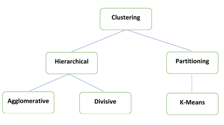
In this blog we shall discuss the K-Means type of clustering, understanding the prerequisites and steps undertaken to model the same using Python.
K-Means Clustering
What is K-means?
- A non-hierarchical approach to forming good clusters.
- For K-Means modelling, the number of clusters needs to be determined before the model is prepared.
- These K values are measured by certain evaluation techniques once the model is run.
- K-means clustering is widely used in large dataset applications.
How does K-means Clustering work?
Pre-Processing of the data
- As this algorithm is based on distance calculation from each observation to the centroids present and this being an iterative process, the data needs to be in a proper format.
- In case the dataset has variables with different units of measures, one should undertake the process of Scaling to bring all the variables into one unit/ measure, for further algorithm processing.
- There are 2 methods of Scaling: Z Scaling and Min-Max Scaling
- Z Scaling:
-
- Features will be rescaled
- Have the properties of a standard normal distribution
- μ=0 and σ=1
-
- Min Max Scaling:
- The data is scaled to a fixed range - 0 to 1.
- The cost of having this bounded range - smaller standard deviations, which can suppress the effect of outliers
Points to remember while Scaling:
- Z Scaling is to be used when the column's variance is very low.
- Min Max Scaling to be used when the variance between columns is high.
- The variance analysis is based on the nature of the dataset and the variables related to it.
Steps followed by K-Means Algorithm
- The first step in this model is to specify the K value.
- Based on this K value, the dataset is partitioned into initial clusters.
- Random centroids are assigned to the dataset from the initial K values which will be away from the original observations.
- Then the model calculates distances from every observation in the cluster to the random centroid. Where the distance value is less and nearer to the random centroid, every observation gets mapped to the centroid. Like this, for all the observations in the dataset, the values are calculated and the observations are assigned suitably. The Euclidean distance metric is the default measure to calculate all distance from the centroid to the observations.
- Once the distances are calculated, random clusters are formed.
- Based on these random clusters, an iterative process of assigning new centroids enables the formation of new clusters. Here the variance is calculated to every observation in the cluster from the centroid. This process runs till the time Heterogeneity between the groups is greater than Homogeneity within the groups i.e SSB > SSW.
Model Evaluation
Silhouette Score:
- This method is also called Indirect model evaluation technique
- The model helps to analyse the correctness of every observation mapped to respective clusters based on distance criteria.
Sil_Width score= (b-a) / MAX(a,b)
where b = distance from the random observation to its neighbouring cluster
a = distance from the random observation to its own cluster
- If the score has a positive value with a range of score between -1 to +1, the cluster mapping of the data point is correct.
- Once this is achieved, we have to get into the Silhouette Score.
- Silhouette Score is the average of Sil_Width score based on the calculation of all the observations in the dataset
- Conclusions drawn:
| Value Tend to | Conclusion |
| +1 | The clusters formed are away from each other. |
| 0 | The clusters are not separable |
| -1 | The model has failed in forming the clusters |
WSS Plot (Elbow Plot):
- WSS Plot also called “Within Sum of Squares” is another solution under the K-Means algorithm which helps to decide the value of K (number of clusters).
- The values taken to plot the WSS plot will be the variance from each observation in the clusters to its centroid, summing up to obtain a value.
The above mentioned theoretical concepts are explained below using Python Programming Language.
K-Means: Python Analysis
Branding of Banks
Let’s consider the banks' dataset and cluster the banks into different segments.
Provide strategic inputs to enhance branding value.
Steps followed in Python
1. Data Collection and Import Libraries
Import the necessary libraries and read data.
Pandas library to be used to read the data and do some basic EDA.
Import matplotlib library which can be used to plot the WSS curve.
To carry out K-Means modelling, import the function from “sklearn.cluster” library
2. Data Handling
Viewing data as a table, performing cleaning activities like checking for spellings, removing blanks and wrong cases, removing invalid values from data, etc.
- Check correctness of imported data using head(). Simultaneously, check and review the shape of the dataset, data type of each variable using info().
- Check duplicate values in the data set. Use describe function to detect outliers in the dataset.
- We observe that the data set is normally distributed. However, the units of variables are different. Hence, we shall scale the data before the K-means algorithm is run.
3. Data Pre-processing
In this section, we will discuss the process of Scaling using the Z-Scaling method to standardise the data for K-Means Algorithm.
Use the Standard Scaler function which is part of the “sklearn” library in Python for scaling the data.
Run Standard Scaler function for all variables except the Bank variable.
There are many ways through which we can select the variables in a matrix format. Using the “iloc” function is one of the methods.
Select a group of columns apart from the Bank variable using the “iloc” function.
4. Modelling and Performance Measure
Start the process of K-Means modelling by assigning random K values. Based on the output, use the model evaluation methodology to understand this dataset's optimum level of clusters.
Assume a random K value of 2. Check whether the clusters are being formed properly.
Let’s check on the Sum of Squares values for cluster 2.
Inertia_ function in Python calculates the Sum of Squares (WSS) distance for all observations in the dataset with a K value of 2.
In order to find out the optimal level of clusters, analyse different Sum of Squares values for different K values.
From the above WSS values, we interpret that while the value of K increases, WSS value decreases.
In order to find the optimal clusters, keep the below points in mind:
- The rate at which the WSS value falls for each cluster - Measuring the difference in the value of WSS from cluster 2 onwards is carried out to understand the fall index of the cluster comprehending the larger variance of the data.
- The most crucial point to remember would be the cluster selection, which would depend on the business objective for the target analysis.
Observation
In the above analysis, we can see maximum data points covered within the first 4 clusters explaining maximum variance in the data basis WSS values. This is re-affirmed since the fall in WSS values from cluster 5 is very less.
We conclude the number of clusters using WSS values and plot the same.
From the above plot, we can see that the fall of WSS values is large enough till cluster 4. This indicates that much of the data's variance gets explained with 4 cluster classification.
Now, using Silhouette Score let us evaluate the cluster formation. As mentioned earlier, the value tending to +1, indicates clusters so formed are correct.
From the above analysis, we can reaffirm the Silhouette score is highest for 4 clusters.
Now append the final list of cluster classification to original data to undertake cluster profiling of the banks.
5. Cluster Profiling
Mean values of each variable are considered in individual clusters along with the frequency numbers for appropriate recommendations to concerned banks in the cluster.
Recommendations
- The banks in Cluster 3 have high DD and Withdrawals but fewer deposits. So, it needs to improve its customers’ Deposits. A relatively large number of customers are visiting these banks. So, they can promote various deposit schemes to these customers.
- Customers in Cluster 3 seem to prefer payment through DD as these banks record the highest DD rate. Banks can check if DD is being made to other banks or to the same bank, and can look to create DD schemes for their own bank so that customers will open their account with these banks and use the DD payment scheme.
- Customers preferring DD payment can go to banks either in Cluster 3 (if they need large space which can manage large crowds probably with more infrastructure facilities), or Cluster 0 (if they want small space where probably quick transactions can happen due to less crowd holding capacity).
- Size of the bank doesn't matter in accommodating a large group of customers inside the bank, as Cluster 0, although having the least Branch Area, has the highest daily walk-ins. So, banks don't need to invest more in occupying large land space. This could mean Customers are visiting throughout the day rather than a large group of customers visiting during a period.
- Cluster 2 has a large area and the proportion of withdrawals and deposits is almost equal. Most of these customers could have a savings account since the withdrawals and DD are less when compared to other clusters. Customers visiting these banks are also lesser than other clusters. These banks can look bringing in more customers and increase the bank deposit by introducing various deposit schemes.
- Deposit is again less, while the withdrawals are much higher for Cluster 1. These banks can also look at introducing new deposit schemes.
- Banks in cluster 0 and 1, need to focus on their infrastructure and banking facilities, since the area is lesser than cluster 3 and 4, whereas daily walk-ins are the highest. These banks can also look for opportunities to cross-sell products to customers.
If you want to pursue a career in data science, upskill with Great Learning's online data science course.
Find Data Science Course in Top Cities in India
Chennai | Bangalore | Hyderabad | Pune | Mumbai | Delhi NCROur Machine Learning Courses
Explore our Machine Learning and AI courses, designed for comprehensive learning and skill development.
| Program Name | Duration |
|---|---|
| MIT No code AI and Machine Learning Course | 12 Weeks |
| MIT Data Science and Machine Learning Course | 12 Weeks |
| Data Science and Machine Learning Course | 12 Weeks |