- What is object detection?
- How is object detection different from object classification?
- Types of object detection algorithms
- Code for object detection using PyTorch
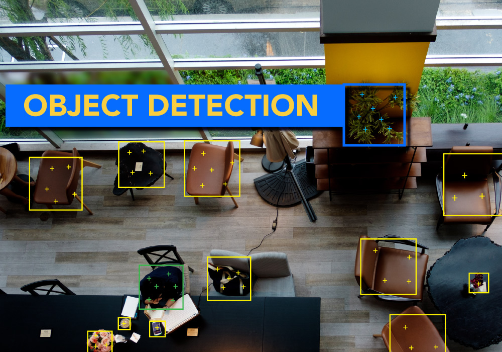
What is object detection?
Object detection is a computer vision technique in which a software system can detect, locate, and trace the object from a given image or video. The special attribute about object detection is that it identifies the class of object (person, table, chair, etc.) and their location-specific coordinates in the given image. The location is pointed out by drawing a bounding box around the object. The bounding box may or may not accurately locate the position of the object. The ability to locate the object inside an image defines the performance of the algorithm used for detection.
These object detection algorithms might be pre-trained or can be trained from scratch. In most use cases, we use pre-trained weights from pre-trained models and then fine-tune them as per our requirements and different use cases.
Labeled data is of paramount importance in these tasks, and every algorithm when put into practice requires a lot of well-labeled data. The algorithms require data of varying nature to function correctly, and this can be done easily by either collecting a lot more samples of data or augmenting the available data in some form.
Data Augmentation is required in such cases when we have particularly limited access to labeled data. Hence, by data augmentation, we create images that are effectively containing the same image but their interpretation is done differently by the algorithms. For instance, let's discuss a particular use case.
Let’s say we are given the task of detecting and classifying different types of fruits. Now the task is to detect both the type of fruit present and to also find the precise coordinates of the fruit in the image. But we have a problem. For training, we have 250 images containing bananas. For apples and oranges, we have only 120 images. This dataset imbalance can be dealt with by Data Augmentation. We can create superficial images by just distorting the existing images. The distortions can be in the form of rotation of images, such that the point of view of the objects in the picture changes. We can try different angles of rotation for the creation of new images. Similarly, we play with the lighting conditions, sharpness, or can even displace the images either vertically or horizontally to create images that will be digitally different from the existing image.
Also Read: Computer Vision: Deep Learning Approach
Now let us see a simple program for object detection using python. The code is very simple if you ignore the underlying architecture.
import cv2
import matplotlib.pyplot as plt
import cvlib
from cvlib.object_detection import draw_bbox
im  =  cv2.imread ('Vegetable - market.jpg')
bbox , label , conf  =  cvlib.detect_common_objects(im)
output_image = draw_bbox (im , bbox , label , conf)
plt.imshow (output_image)
plt.show()
Here cvlib is the library that has an object detection function for common objects. The model is trained to detect a variety of common objects like fruits, people, cars, etc.
Every detected object can be seen in the resulting image with a bounding box around it. This a picture of a vegetable market we picked up randomly from the internet. You can experiment with your own image. Just change the name of the image in the given code and you are good to go.
Another simple use case of object detection is face detection. Face detection is a specialized case of object detection in images or videos which is a collection of images in sequence. In a general object detection algorithm, the task is to identify a particular class of objects whether it be dogs, cats, trees, fruit cars, etc.
In face detection, we have a database of images with faces and the aspect ratio of various distances. Facial feature data is stored in the database.
When a new object comes in, its features are compared to that of faces stored in the database. Any feature mismatch disqualifies the image as a face. If all features are matched then a bounding box is drawn around the detected face.
We would be using the same concept in which we will store all the attributes of a face in XML file. We would read each frame of our webcam and then, if a face is found in the particular frame we will draw a bounding box around the face.
Also Read: Datasets for Computer Vision using Deep Learning
For this we will require the OpenCV module and harrcascade_default.xml
We begin with importing the cv2 module. If you have not already installed it, you can do so by doing the following.
!pip install opencv-python
import cv2
We then load the XML file which has all data about the facial features.
# Load the cascade
face_cascade = cv2.CascadeClassifier('haarcascade_frontalface_default.xml')
We then start capturing the video using object detection.
# To capture video from a webcam.
cap = cv2.VideoCapture(0)
# To use a video file as input
# cap = cv2.VideoCapture('filename.mp4')
Until we press escape the webcam will be functional. We read each frame and then convert that frame to a grayscale image.
while True:
# Read the frame
_, img = cap.read()
# Convert to grayscale
gray = cv2.cvtColor(img, cv2.COLOR_BGR2GRAY)
We then call the detectMultiScale function of OpenCV to detect faces in the frame. It detects multiple faces so if you hold a mobile phone with faces in it in front of the webcam it detects them as well.
# Detect the faces
faces = face_cascade.detectMultiScale(gray, 1.1, 4)
# Draw the rectangle around each face
for (x, y, w, h) in faces:
cv2.rectangle(img, (x, y), (x+w, y+h), (255, 0, 0), 2)
# Display
cv2.imshow('img', img)
# Stop if escape key is pressed
k = cv2.waitKey(30) & 0xff
if k==27:
break
# Release the VideoCapture object
cap.release()
How is object detection different from object classification?
Object classification is a traditional computer vision task that is effectively determining the class of the object in an image. Object classification finds out what the object in a given picture or video is. There is a probability score associated with the results so that we can get the confidence scores of the results.
Let’s perform object detection on the mnist dataset and fashion mnist data sets to give you more clarity on the topic.
import tensorflow as tf
mnist = tf.keras.datasets.mnist
(x_train, y_train), (x_test, y_test) = mnist.load_data()
x_train, x_test = x_train / 255.0, x_test / 255.0
model = tf.keras.models.Sequential([
tf.keras.layers.Flatten(input_shape=(28, 28)),
tf.keras.layers.Dense(128, activation='relu'),
tf.keras.layers.Dropout(0.2),
tf.keras.layers.Dense(10)
])
predictions = model(x_train[:1]).numpy()
predictions
Output:
array([[-0.63204   ,  0.29606453,  0.24910979,  0.28201205, -0.17138952,
0.3396452 ,  0.37800127, -0.9318958 ,  0.0439647 , -0.0467336 ]],
dtype=float32)
tf.nn.softmax(predictions).numpy()
Output:
array([[0.05021724, 0.12703504, 0.12120801, 0.12526236, 0.07959959,
0.13269372, 0.1378822 , 0.03720722, 0.09872746, 0.09016712]],
dtype=float32)
loss_fn = tf.keras.losses.SparseCategoricalCrossentropy(from_logits=True)
loss_fn(y_train[:1], predictions).numpy()
model.compile(optimizer='adam',
         loss=loss_fn,
         metrics=['accuracy'])
model.fit(x_train, y_train, epochs=20)
Ouput:
Epoch 1/20
1875/1875 [==============================] - 4s 2ms/step - loss: 0.0672 - accuracy: 0.9791
Epoch 2/20
1875/1875 [==============================] - 3s 2ms/step - loss: 0.0580 - accuracy: 0.9811
Epoch 3/20
1875/1875 [==============================] - 4s 2ms/step - loss: 0.0537 - accuracy: 0.9829
Epoch 4/20
1875/1875 [==============================] - 3s 2ms/step - loss: 0.0472 - accuracy: 0.9851
Epoch 5/20
1875/1875 [==============================] - 4s 2ms/step - loss: 0.0446 - accuracy: 0.9855
Epoch 6/20
1875/1875 [==============================] - 4s 2ms/step - loss: 0.0399 - accuracy: 0.9870
Epoch 7/20
1875/1875 [==============================] - 4s 2ms/step - loss: 0.0403 - accuracy: 0.9857
Epoch 8/20
1875/1875 [==============================] - 4s 2ms/step - loss: 0.0351 - accuracy: 0.9885
Epoch 9/20
1875/1875 [==============================] - 4s 2ms/step - loss: 0.0343 - accuracy: 0.9886
Epoch 10/20
1875/1875 [==============================] - 4s 2ms/step - loss: 0.0347 - accuracy: 0.9880
Epoch 11/20
1875/1875 [==============================] - 4s 2ms/step - loss: 0.0296 - accuracy: 0.9901
Epoch 12/20
1875/1875 [==============================] - 4s 2ms/step - loss: 0.0285 - accuracy: 0.9901
Epoch 13/20
1875/1875 [==============================] - 4s 2ms/step - loss: 0.0288 - accuracy: 0.9902
Epoch 14/20
1875/1875 [==============================] - 3s 2ms/step - loss: 0.0268 - accuracy: 0.9908
Epoch 15/20
1875/1875 [==============================] - 4s 2ms/step - loss: 0.0277 - accuracy: 0.9901
Epoch 16/20
1875/1875 [==============================] - 4s 2ms/step - loss: 0.0228 - accuracy: 0.9919
Epoch 17/20
1875/1875 [==============================] - 4s 2ms/step - loss: 0.0236 - accuracy: 0.9918
Epoch 18/20
1875/1875 [==============================] - 4s 2ms/step - loss: 0.0233 - accuracy: 0.9920
Epoch 19/20
1875/1875 [==============================] - 4s 2ms/step - loss: 0.0230 - accuracy: 0.9920
Epoch 20/20
1875/1875 [==============================] - 4s 2ms/step - loss: 0.0227 - accuracy: 0.9919
<tensorflow.python.keras.callbacks.History at 0x7fa0f06cd390>
model.evaluate(x_test, y_test, verbose=2)Output:
313/313 - 0s - loss: 0.0765 - accuracy: 0.9762
[0.07645969837903976, 0.9761999845504761]
probability_model = tf.keras.Sequential([
model,
tf.keras.layers.Softmax()
])
probability_model(x_test[:5])
Ouput:
<tf.Tensor: shape=(5, 10), dtype=float32, numpy=
array([[3.9212882e-12, 2.1834714e-19, 1.9253871e-10, 2.2876110e-07,
9.0482010e-19, 1.1011923e-11, 2.5250806e-23, 9.9999976e-01,
1.7883041e-12, 1.3832281e-09],
[1.4191020e-17, 1.3323700e-10, 1.0000000e+00, 7.2097401e-16,
6.5754260e-37, 2.3290989e-16, 8.8370928e-17, 1.0187791e-29,
2.0311796e-18, 0.0000000e+00],
[7.0981394e-17, 9.9999857e-01, 5.5766418e-07, 7.3810041e-11,
4.1638457e-09, 5.4865166e-12, 1.6843820e-12, 7.9530673e-07,
2.9518892e-08, 2.5004247e-15],
[9.9999964e-01, 6.0739493e-21, 1.9297003e-07, 4.0246032e-13,
1.5357564e-12, 2.8772764e-08, 9.8391717e-10, 4.7179654e-08,
3.7541407e-17, 7.9969936e-10],
[9.2232035e-14, 2.7456325e-20, 1.8037905e-14, 7.4756340e-18,
9.9999642e-01, 7.5487475e-15, 6.5344392e-12, 6.5705713e-08,
7.8566824e-13, 3.4821376e-06]], dtype=float32)>
In the above example we did a use case on object classification using MNIST.
Let’s see another example, using the fashion mnist dataset.
# TensorFlow and tf.keras
#based on tensorflow examples from google
import tensorflow as tf
from tensorflow import keras
# Helper libraries
import numpy as np
import matplotlib.pyplot as plt
fashion_mnist = keras.datasets.fashion_mnist
(train_images, train_labels), (test_images, test_labels) = fashion_mnist.load_data()
class_names = [‘T-shirt/top’, ‘Trouser’, ‘Pullover’, ‘Dress’, ‘Coat’,
        	‘Sandal’, ‘Shirt’, ‘Sneaker’, ‘Bag’, ‘Ankle boot’]
plt.figure()
plt.imshow(train_images[0])
plt.colorbar()
plt.grid(False)
plt.show()
train_images[10]
Ouput:
array([[0.    , 0.    , 0.    , 0.    , 0.        ,
 	0.    , 0.    , 0.04313725, 0.55686275, 0.78431373,
 	0.41568627, 0.    , 0.    , 0.    , 0.    ,
 	0.    , 0.    , 0.    , 0.33333333, 0.7254902 ,
 	0.43921569, 0.    , 0.    , 0.    , 0.    ,
 	0.    , 0.    , 0.    ],
	[0.    , 0.    , 0.    , 0.    , 0.    ,
 	0.    , 0.59607843, 0.83921569, 0.85098039, 0.76078431,
 	0.9254902 , 0.84705882, 0.73333333, 0.58431373, 0.52941176,
 	0.6   , 0.82745098, 0.85098039, 0.90588235, 0.80392157,
 	0.85098039, 0.7372549 , 0.13333333, 0.    , 0.    ,
 	0.    , 0.    , 0.    ],
	[0.    , 0.    , 0.    , 0.    , 0.    ,
 	0.25882353, 0.7254902 , 0.65098039, 0.70588235, 0.70980392,
 	0.74509804, 0.82745098, 0.86666667, 0.77254902, 0.57254902,
 	0.77647059, 0.80784314, 0.74901961, 0.65882353, 0.74509804,
 	0.6745098 , 0.7372549 , 0.68627451, 0.    , 0.    ,
 	0.    , 0.    , 0.    ],
    [0.    , 0.    , 0.    , 0.    , 0.    ,
 	0.52941176, 0.6   , 0.62745098, 0.68627451, 0.70588235,
 	0.66666667, 0.72941176, 0.73333333, 0.74509804, 0.7372549 ,
 	0.74509804, 0.73333333, 0.68235294, 0.76470588, 0.7254902 ,
 	0.68235294, 0.63137255, 0.68627451, 0.23137255, 0.    ,
 	0.    , 0.    , 0.    ],
	[0.    , 0.    , 0.    , 0.    , 0.    ,
 	0.63137255, 0.57647059, 0.62745098, 0.66666667, 0.69803922,
 	0.69411765, 0.70588235, 0.65882353, 0.67843137, 0.68235294,
 	0.67058824, 0.7254902 , 0.72156863, 0.7254902 , 0.6745098 ,
 	0.67058824, 0.64313725, 0.68235294, 0.47058824, 0.    ,
 	0.    , 0.    , 0.    ],
	[0.    , 0.    , 0.    , 0.    , 0.00784314,
 	0.68627451, 0.57254902, 0.56862745, 0.65882353, 0.69803922,
	0.70980392, 0.7254902 , 0.70588235, 0.72156863, 0.69803922,
 	0.70196078, 0.73333333, 0.74901961, 0.75686275, 0.74509804,
 	0.70980392, 0.67058824, 0.6745098 , 0.61960784, 0.    ,
 	0.    , 0.    , 0.    ],
	[0.     , 0.    , 0.    , 0.   , 0.1372549 ,
 	0.69411765, 0.60784314, 0.54901961, 0.59215686, 0.6745098 ,
 	0.74901961, 0.73333333, 0.72941176, 0.73333333, 0.72941176,
 	0.73333333, 0.71372549, 0.74901961, 0.76078431, 0.7372549 ,
 	0.70588235, 0.63137255, 0.63137255, 0.7254902 , 0.    ,
 	0.    , 0.    , 0.    ],
	[0.    , 0.    , 0.    , 0.    , 0.23137255,
 	0.66666667, 0.6   , 0.55294118, 0.47058824, 0.60392157,
    0.62745098, 0.63137255, 0.6745098 , 0.65882353, 0.65098039,
 	0.63137255, 0.64705882, 0.6745098 , 0.66666667, 0.64313725,
 	0.54509804, 0.58431373, 0.63529412, 0.65098039, 0.08235294,
 	0.    , 0.    , 0.    ],
	[0.        , 0.    , 0.    , 0.   , 0.30980392,
 	0.56862745, 0.62745098, 0.83921569, 0.48235294, 0.50196078,
 	0.6   , 0.62745098, 0.64313725, 0.61960784, 0.61568627,
 	0.60392157, 0.60784314, 0.66666667, 0.64705882, 0.55294118,
 	0.76470588, 0.75686275, 0.59607843, 0.65098039, 0.23921569,
 	0.    , 0.    , 0.    ],
	[0.    , 0.    , 0.    , 0.    , 0.39215686,
 	0.61568627, 0.88235294, 0.96078431, 0.68627451, 0.44313725,
 	0.68235294, 0.61960784, 0.61960784, 0.62745098, 0.60784314,
 	0.62745098, 0.64313725, 0.69803922, 0.7372549 , 0.52941176,
 	0.7254902 , 0.94117647, 0.78823529, 0.6745098 , 0.42352941,
 	0.    , 0.    , 0.    ],
	[0.    , 0.    , 0.    , 0.        , 0.    ,
 	0.12156863, 0.68235294, 0.10980392, 0.49411765, 0.6   ,
 	0.65098039, 0.59607843, 0.61960784, 0.61960784, 0.62745098,
 	0.63137255, 0.61568627, 0.65882353, 0.74901961, 0.7372549 ,
 	0.07058824, 0.51764706, 0.62352941, 0.02745098, 0.    ,
 	0.    , 0.    , 0.    ],
	[0.    , 0.    , 0.    , 0.    , 0.    ,
 	0.    , 0.    , 0.    , 0.32156863, 0.73333333,
 	0.62352941, 0.6   , 0.61568627, 0.61960784, 0.63529412,
 	0.64313725, 0.64313725, 0.60392157, 0.73333333, 0.74509804,
 	0.    , 0.    , 0.    , 0.     , 0.    ,
 	0.    , 0.    , 0.    ],
	[0.    , 0.    , 0.    , 0.        , 0.00392157,
 	0.01176471, 0.01960784, 0.    , 0.14509804, 0.68627451,
 	0.61960784, 0.60784314, 0.63529412, 0.61960784, 0.62745098,
 	0.63529412, 0.64705882, 0.6   , 0.69411765, 0.80392157,
 	0.    , 0.    , 0.01176471, 0.01176471, 0.    ,
 	0.    , 0.    , 0.    ],
	[0.    , 0.    , 0.    , 0.    , 0.    ,
 	0.    , 0.00392157, 0.    , 0.09803922, 0.68627451,
 	0.59607843, 0.62745098, 0.61960784, 0.63137255, 0.62745098,
 	0.64313725, 0.64313725, 0.63137255, 0.65098039, 0.78431373,
 	0.    , 0.    , 0.00392157, 0.    , 0.    ,
 	0.    , 0.    , 0.    ],
	[0.    , 0.    , 0.    , 0.    , 0.    ,
 	0.    , 0.01568627, 0.    , 0.11764706, 0.67058824,
	0.57647059, 0.64313725, 0.60784314, 0.64705882, 0.63137255,
 	0.64705882, 0.63529412, 0.66666667, 0.64313725, 0.63529412,
 	0.    , 0.   , 0.00784314, 0.    , 0.    ,
 	0.    , 0.    , 0.    ],
	[0.     , 0.    , 0.    , 0.    , 0.    ,
 	0.    , 0.01568627, 0.    , 0.22352941, 0.65098039,
 	0.60784314, 0.64313725, 0.65098039, 0.63137255, 0.63137255,
 	0.64313725, 0.65490196, 0.64705882, 0.64705882, 0.63529412,
 	0.10980392, 0.    , 0.01176471, 0.    , 0.    ,
 	0.    , 0.    , 0.    ],
	[0.    , 0.    , 0.    , 0.    , 0.    ,
 	0.    , 0.01176471, 0.    , 0.44705882, 0.63137255,
    0.63137255, 0.65098039, 0.62352941, 0.65882353, 0.63137255,
 	0.63137255, 0.6745098 , 0.63529412, 0.64705882, 0.67058824,
 	0.19607843, 0.   , 0.01960784, 0.    , 0.    ,
 	0.    , 0.    , 0.    ],
	[0.        , 0.    , 0.    , 0.    , 0.    ,
 	0.    , 0.00392157, 0.    , 0.58431373, 0.61568627,
 	0.65490196, 0.6745098 , 0.62352941, 0.6745098 , 0.64313725,
 	0.63137255, 0.6745098 , 0.66666667, 0.62745098, 0.67058824,
 	0.34901961, 0.    , 0.01568627, 0.    , 0.    ,
 	0.    , 0.    , 0.    ],
	[0.    , 0.    , 0.   , 0.    , 0.    ,
 	0.00784314, 0.    , 0.01568627, 0.67058824, 0.64313725,
 	0.65098039, 0.67843137, 0.62352941, 0.70196078, 0.65098039,
 	0.62745098, 0.68235294, 0.65490196, 0.63529412, 0.65098039,
 	0.50196078, 0.        , 0.00784314, 0.    , 0.    ,
 	0.    , 0.    , 0.    ],
	[0.    , 0.    , 0.    , 0.    , 0.    ,
 	0.01176471, 0.    , 0.07058824, 0.59607843, 0.67843137,
 	0.62745098, 0.70196078, 0.60392157, 0.70980392, 0.65098039,
 	0.64313725, 0.68627451, 0.66666667, 0.65098039, 0.66666667,
 	0.64313725, 0.    , 0.    , 0.00392157, 0.    ,
 	0.    , 0.    , 0.    ],
	[0.    , 0.    , 0.   , 0.    , 0.    ,
 	0.01568627, 0.    , 0.18431373, 0.64705882, 0.6745098 ,
 	0.65490196, 0.7254902 , 0.6   , 0.73333333, 0.67843137,
 	0.64705882, 0.68235294, 0.70196078, 0.65098039, 0.65098039,
 	0.61960784, 0.01960784, 0.    , 0.01176471, 0.    ,
 	0.    , 0.    , 0.    ],
	[0.    , 0.    , 0.    , 0.    , 0.    ,
 	0.01568627, 0.    , 0.34117647, 0.70588235, 0.63529412,
 	0.70196078, 0.70196078, 0.61568627, 0.74901961, 0.71372549,
 	0.64705882, 0.65882353, 0.74509804, 0.67843137, 0.64705882,
 	0.65098039, 0.07843137, 0.    , 0.01568627, 0.    ,
 	0.    , 0.    , 0.    ],
	[0.    , 0.    , 0.        , 0.    , 0.    ,
 	0.01568627, 0.    , 0.41176471, 0.73333333, 0.61568627,
 	0.76078431, 0.68627451, 0.63137255, 0.74509804, 0.72156863,
 	0.66666667, 0.61960784, 0.80392157, 0.69411765, 0.65882353,
 	0.67058824, 0.17254902, 0.    , 0.01568627, 0.    ,
 	0.    , 0.    , 0.    ],
	[0.    , 0.    , 0.    , 0.    , 0.    ,
 	0.01960784, 0.    , 0.54117647, 0.70980392, 0.61960784,
	0.80392157, 0.62745098, 0.65490196, 0.74509804, 0.77647059,
 	0.65490196, 0.59607843, 0.85490196, 0.72941176, 0.66666667,
 	0.6745098 , 0.22352941, 0.    , 0.01960784, 0.    ,
 	0.    , 0.    , 0.    ],
	[0.     , 0.    , 0.        , 0.    , 0.    ,
 	0.01960784, 0.    , 0.52941176, 0.68235294, 0.65490196,
 	0.78039216, 0.60784314, 0.65098039, 0.78823529, 0.85882353,
 	0.64705882, 0.61960784, 0.85490196, 0.7372549 , 0.65490196,
 	0.68627451, 0.21960784, 0.    , 0.02745098, 0.    ,
 	0.    , 0.    , 0.    ],
	[0.    , 0.    , 0.    , 0.    , 0.    ,
 	0.01960784, 0.    , 0.50588235, 0.67058824, 0.6745098 ,
    0.69411765, 0.6       , 0.62352941, 0.80784314, 0.84705882,
 	0.58039216, 0.61568627, 0.80784314, 0.74509804, 0.64705882,
 	0.68627451, 0.18823529, 0.    , 0.01960784, 0.    ,
 	0.    , 0.    , 0.    ],
	[0.        , 0.    , 0.    , 0.    , 0.    ,
 	0.01960784, 0.    , 0.65490196, 0.73333333, 0.71372549,
 	0.77647059, 0.76078431, 0.78431373, 0.88627451, 0.94117647,
 	0.72156863, 0.80784314, 1.    , 0.77254902, 0.69803922,
 	0.70196078, 0.16470588, 0.    , 0.01960784, 0.    ,
 	0.    , 0.    , 0.    ],
	[0.    , 0.    , 0.    , 0.    , 0.    ,
 	0.01176471, 0.    , 0.45098039, 0.52941176, 0.44313725,
 	0.41568627, 0.33333333, 0.32156863, 0.42352941, 0.52156863,
 	0.3254902 , 0.35294118, 0.4745098 , 0.47058824, 0.43137255,
 	0.61960784, 0.07058824, 0.    , 0.01176471, 0.    ,
 	0.    , 0.    , 0.    ]])
#scale pixel values between 0 and 1
x=255.0
train_images = train_images / x
test_images = test_images / x
plt.figure(figsize=(15,15))
j=np.random.randint(0,1000,100)
y=1
for i in range(100):
plt.subplot(10,10,i+y)
plt.xticks([])
plt.yticks([])
plt.grid(False)
plt.imshow(train_images[j[i]], cmap=plt.cm.binary)
plt.xlabel(class_names[train_labels[i]])
plt.show()
#after scaling
Train_images[10]
Output:
array([[0.00000000e+00, 0.00000000e+00, 0.00000000e+00, 0.00000000e+00,
 	0.00000000e+00, 0.00000000e+00, 0.00000000e+00, 6.63394924e-07,
 	8.56382538e-06, 1.20617259e-05, 6.39271472e-06, 0.00000000e+00,
 	0.00000000e+00, 0.00000000e+00, 0.00000000e+00, 0.00000000e+00,
 	0.00000000e+00, 0.00000000e+00, 5.12623350e-06, 1.11570964e-05,
        6.75456649e-06, 0.00000000e+00, 0.00000000e+00, 0.00000000e+00,
 	0.00000000e+00, 0.00000000e+00, 0.00000000e+00, 0.00000000e+00],
	[0.00000000e+00, 0.00000000e+00, 0.00000000e+00, 0.00000000e+00,
 	0.00000000e+00, 0.00000000e+00, 9.16691167e-06, 1.29060467e-05,
 	1.30869726e-05, 1.16998741e-05, 1.42328365e-05, 1.30266640e-05,
 	1.12777137e-05, 8.98598578e-06, 8.14166497e-06, 9.22722030e-06,
 	1.27251208e-05, 1.30869726e-05, 1.39312934e-05, 1.23632690e-05,
 	1.30869726e-05, 1.13380223e-05, 2.05049340e-06, 0.00000000e+00,
 	0.00000000e+00, 0.00000000e+00, 0.00000000e+00, 0.00000000e+00],
	[0.00000000e+00, 0.00000000e+00, 0.00000000e+00, 0.00000000e+00,
 	0.00000000e+00, 3.98036954e-06, 1.11570964e-05, 1.00112325e-05,
 	1.08555533e-05, 1.09158619e-05, 1.14586396e-05, 1.27251208e-05,
 	1.33282071e-05, 1.18808000e-05, 8.80505989e-06, 1.19411086e-05,
 	1.24235777e-05, 1.15189482e-05, 1.01318497e-05, 1.14586396e-05,
 	1.03730843e-05, 1.13380223e-05, 1.05540101e-05, 0.00000000e+00,
 	0.00000000e+00, 0.00000000e+00, 0.00000000e+00, 0.00000000e+00],
	[0.00000000e+00, 0.00000000e+00, 0.00000000e+00, 0.00000000e+00,
 	0.00000000e+00, 8.14166497e-06, 9.22722030e-06, 9.64938071e-06,
 	1.05540101e-05, 1.08555533e-05, 1.02524670e-05, 1.12174051e-05,
 	1.12777137e-05, 1.14586396e-05, 1.13380223e-05, 1.14586396e-05,
 	1.12777137e-05, 1.04937015e-05, 1.17601827e-05, 1.11570964e-05,
 	1.04937015e-05, 9.70968934e-06, 1.05540101e-05, 3.55820914e-06,
 	0.00000000e+00, 0.00000000e+00, 0.00000000e+00, 0.00000000e+00],
	[0.00000000e+00, 0.00000000e+00, 0.00000000e+00, 0.00000000e+00,
 	0.00000000e+00, 9.70968934e-06, 8.86536852e-06, 9.64938071e-06,
	1.02524670e-05, 1.07349360e-05, 1.06746274e-05, 1.08555533e-05,
 	1.01318497e-05, 1.04333929e-05, 1.04937015e-05, 1.03127756e-05,
 	1.11570964e-05, 1.10967878e-05, 1.11570964e-05, 1.03730843e-05,
 	1.03127756e-05, 9.89061522e-06, 1.04937015e-05, 7.23703553e-06,
 	0.00000000e+00, 0.00000000e+00, 0.00000000e+00, 0.00000000e+00],
	[0.00000000e+00, 0.00000000e+00, 0.00000000e+00, 0.00000000e+00,
 	1.20617259e-07, 1.05540101e-05, 8.80505989e-06, 8.74475126e-06,
 	1.01318497e-05, 1.07349360e-05, 1.09158619e-05, 1.11570964e-05,
 	1.08555533e-05, 1.10967878e-05, 1.07349360e-05, 1.07952447e-05,
 	1.12777137e-05, 1.15189482e-05, 1.16395655e-05, 1.14586396e-05,
 	1.09158619e-05, 1.03127756e-05, 1.03730843e-05, 9.52876345e-06,
 	0.00000000e+00, 0.00000000e+00, 0.00000000e+00, 0.00000000e+00],
	[0.00000000e+00, 0.00000000e+00, 0.00000000e+00, 0.00000000e+00,
 	2.11080203e-06, 1.06746274e-05, 9.34783756e-06, 8.44320812e-06,
    9.10660304e-06, 1.03730843e-05, 1.15189482e-05, 1.12777137e-05,
 	1.12174051e-05, 1.12777137e-05, 1.12174051e-05, 1.12777137e-05,
 	1.09761706e-05, 1.15189482e-05, 1.16998741e-05, 1.13380223e-05,
 	1.08555533e-05, 9.70968934e-06, 9.70968934e-06, 1.11570964e-05,
 	0.00000000e+00, 0.00000000e+00, 0.00000000e+00, 0.00000000e+00],
	[0.00000000e+00, 0.00000000e+00, 0.00000000e+00, 0.00000000e+00,
 	3.55820914e-06, 1.02524670e-05, 9.22722030e-06, 8.50351675e-06,
 	7.23703553e-06, 9.28752893e-06, 9.64938071e-06, 9.70968934e-06,
 	1.03730843e-05, 1.01318497e-05, 1.00112325e-05, 9.70968934e-06,
 	9.95092385e-06, 1.03730843e-05, 1.02524670e-05, 9.89061522e-06,
 	8.38289949e-06, 8.98598578e-06, 9.76999796e-06, 1.00112325e-05,
 	1.26648122e-06, 0.00000000e+00, 0.00000000e+00, 0.00000000e+00],
	[0.00000000e+00, 0.00000000e+00, 0.00000000e+00, 0.00000000e+00,
	4.76438172e-06, 8.74475126e-06, 9.64938071e-06, 1.29060467e-05,
 	7.41796142e-06, 7.71950456e-06, 9.22722030e-06, 9.64938071e-06,
 	9.89061522e-06, 9.52876345e-06, 9.46845482e-06, 9.28752893e-06,
 	9.34783756e-06, 1.02524670e-05, 9.95092385e-06, 8.50351675e-06,
 	1.17601827e-05, 1.16395655e-05, 9.16691167e-06, 1.00112325e-05,
 	3.67882639e-06, 0.00000000e+00, 0.00000000e+00, 0.00000000e+00],
	[0.00000000e+00, 0.00000000e+00, 0.00000000e+00, 0.00000000e+00,
 	6.03086294e-06, 9.46845482e-06, 1.35694416e-05, 1.47756142e-05,
 	1.05540101e-05, 6.81487512e-06, 1.04937015e-05, 9.52876345e-06,
 	9.52876345e-06, 9.64938071e-06, 9.34783756e-06, 9.64938071e-06,
 	9.89061522e-06, 1.07349360e-05, 1.13380223e-05, 8.14166497e-06,
 	1.11570964e-05, 1.44740711e-05, 1.21220345e-05, 1.03730843e-05,
 	6.51333198e-06, 0.00000000e+00, 0.00000000e+00, 0.00000000e+00],
	[0.00000000e+00, 0.00000000e+00, 0.00000000e+00, 0.00000000e+00,
 	0.00000000e+00, 1.86956751e-06, 1.04937015e-05, 1.68864162e-06,
 	7.59888731e-06, 9.22722030e-06, 1.00112325e-05, 9.16691167e-06,
 	9.52876345e-06, 9.52876345e-06, 9.64938071e-06, 9.70968934e-06,
 	9.46845482e-06, 1.01318497e-05, 1.15189482e-05, 1.13380223e-05,
 	1.08555533e-06, 7.96073908e-06, 9.58907208e-06, 4.22160406e-07,
 	0.00000000e+00, 0.00000000e+00, 0.00000000e+00, 0.00000000e+00],
	[0.00000000e+00, 0.00000000e+00, 0.00000000e+00, 0.00000000e+00,
 	0.00000000e+00, 0.00000000e+00, 0.00000000e+00, 0.00000000e+00,
 	4.94530761e-06, 1.12777137e-05, 9.58907208e-06, 9.22722030e-06,
 	9.46845482e-06, 9.52876345e-06, 9.76999796e-06, 9.89061522e-06,
 	9.89061522e-06, 9.28752893e-06, 1.12777137e-05, 1.14586396e-05,
 	0.00000000e+00, 0.00000000e+00, 0.00000000e+00, 0.00000000e+00,
	0.00000000e+00, 0.00000000e+00, 0.00000000e+00, 0.00000000e+00],
	[0.00000000e+00, 0.00000000e+00, 0.00000000e+00, 0.00000000e+00,
 	6.03086294e-08, 1.80925888e-07, 3.01543147e-07, 0.00000000e+00,
 	2.23141929e-06, 1.05540101e-05, 9.52876345e-06, 9.34783756e-06,
 	9.76999796e-06, 9.52876345e-06, 9.64938071e-06, 9.76999796e-06,
 	9.95092385e-06, 9.22722030e-06, 1.06746274e-05, 1.23632690e-05,
 	0.00000000e+00, 0.00000000e+00, 1.80925888e-07, 1.80925888e-07,
 	0.00000000e+00, 0.00000000e+00, 0.00000000e+00, 0.00000000e+00],
	[0.00000000e+00, 0.00000000e+00, 0.00000000e+00, 0.00000000e+00,
 	0.00000000e+00, 0.00000000e+00, 6.03086294e-08, 0.00000000e+00,
 	1.50771574e-06, 1.05540101e-05, 9.16691167e-06, 9.64938071e-06,
 	9.52876345e-06, 9.70968934e-06, 9.64938071e-06, 9.89061522e-06,
 	9.89061522e-06, 9.70968934e-06, 1.00112325e-05, 1.20617259e-05,
 	0.00000000e+00, 0.00000000e+00, 6.03086294e-08, 0.00000000e+00,
 	0.00000000e+00, 0.00000000e+00, 0.00000000e+00, 0.00000000e+00],
	[0.00000000e+00, 0.00000000e+00, 0.00000000e+00, 0.00000000e+00,
 	0.00000000e+00, 0.00000000e+00, 2.41234518e-07, 0.00000000e+00,
 	1.80925888e-06, 1.03127756e-05, 8.86536852e-06, 9.89061522e-06,
 	9.34783756e-06, 9.95092385e-06, 9.70968934e-06, 9.95092385e-06,
 	9.76999796e-06, 1.02524670e-05, 9.89061522e-06, 9.76999796e-06,
 	0.00000000e+00, 0.00000000e+00, 1.20617259e-07, 0.00000000e+00,
 	0.00000000e+00, 0.00000000e+00, 0.00000000e+00, 0.00000000e+00],
	[0.00000000e+00, 0.00000000e+00, 0.00000000e+00, 0.00000000e+00,
 	0.00000000e+00, 0.00000000e+00, 2.41234518e-07, 0.00000000e+00,
 	3.43759188e-06, 1.00112325e-05, 9.34783756e-06, 9.89061522e-06,
 	1.00112325e-05, 9.70968934e-06, 9.70968934e-06, 9.89061522e-06,
 	1.00715411e-05, 9.95092385e-06, 9.95092385e-06, 9.76999796e-06,
 	1.68864162e-06, 0.00000000e+00, 1.80925888e-07, 0.00000000e+00,
	0.00000000e+00, 0.00000000e+00, 0.00000000e+00, 0.00000000e+00],
	[0.00000000e+00, 0.00000000e+00, 0.00000000e+00, 0.00000000e+00,
 	0.00000000e+00, 0.00000000e+00, 1.80925888e-07, 0.00000000e+00,
 	6.87518375e-06, 9.70968934e-06, 9.70968934e-06, 1.00112325e-05,
        9.58907208e-06, 1.01318497e-05, 9.70968934e-06, 9.70968934e-06,
 	1.03730843e-05, 9.76999796e-06, 9.95092385e-06, 1.03127756e-05,
 	3.01543147e-06, 0.00000000e+00, 3.01543147e-07, 0.00000000e+00,
 	0.00000000e+00, 0.00000000e+00, 0.00000000e+00, 0.00000000e+00],
	[0.00000000e+00, 0.00000000e+00, 0.00000000e+00, 0.00000000e+00,
 	0.00000000e+00, 0.00000000e+00, 6.03086294e-08, 0.00000000e+00,
 	8.98598578e-06, 9.46845482e-06, 1.00715411e-05, 1.03730843e-05,
 	9.58907208e-06, 1.03730843e-05, 9.89061522e-06, 9.70968934e-06,
 	1.03730843e-05, 1.02524670e-05, 9.64938071e-06, 1.03127756e-05,
 	5.36746802e-06, 0.00000000e+00, 2.41234518e-07, 0.00000000e+00,
 	0.00000000e+00, 0.00000000e+00, 0.00000000e+00, 0.00000000e+00],
	[0.00000000e+00, 0.00000000e+00, 0.00000000e+00, 0.00000000e+00,
 	0.00000000e+00, 1.20617259e-07, 0.00000000e+00, 2.41234518e-07,
 	1.03127756e-05, 9.89061522e-06, 1.00112325e-05, 1.04333929e-05,
 	9.58907208e-06, 1.07952447e-05, 1.00112325e-05, 9.64938071e-06,
 	1.04937015e-05, 1.00715411e-05, 9.76999796e-06, 1.00112325e-05,
 	7.71950456e-06, 0.00000000e+00, 1.20617259e-07, 0.00000000e+00,
 	0.00000000e+00, 0.00000000e+00, 0.00000000e+00, 0.00000000e+00],
	[0.00000000e+00, 0.00000000e+00, 0.00000000e+00, 0.00000000e+00,
 	0.00000000e+00, 1.80925888e-07, 0.00000000e+00, 1.08555533e-06,
 	9.16691167e-06, 1.04333929e-05, 9.64938071e-06, 1.07952447e-05,
 	9.28752893e-06, 1.09158619e-05, 1.00112325e-05, 9.89061522e-06,
 	1.05540101e-05, 1.02524670e-05, 1.00112325e-05, 1.02524670e-05,
	9.89061522e-06, 0.00000000e+00, 0.00000000e+00, 6.03086294e-08,
 	0.00000000e+00, 0.00000000e+00, 0.00000000e+00, 0.00000000e+00],
	[0.00000000e+00, 0.00000000e+00, 0.00000000e+00, 0.00000000e+00,
 	0.00000000e+00, 2.41234518e-07, 0.00000000e+00, 2.83450558e-06,
 	9.95092385e-06, 1.03730843e-05, 1.00715411e-05, 1.11570964e-05,
 	9.22722030e-06, 1.12777137e-05, 1.04333929e-05, 9.95092385e-06,
 	1.04937015e-05, 1.07952447e-05, 1.00112325e-05, 1.00112325e-05,
 	9.52876345e-06, 3.01543147e-07, 0.00000000e+00, 1.80925888e-07,
 	0.00000000e+00, 0.00000000e+00, 0.00000000e+00, 0.00000000e+00],
	[0.00000000e+00, 0.00000000e+00, 0.00000000e+00, 0.00000000e+00,
 	0.00000000e+00, 2.41234518e-07, 0.00000000e+00, 5.24685076e-06,
 	1.08555533e-05, 9.76999796e-06, 1.07952447e-05, 1.07952447e-05,
 	9.46845482e-06, 1.15189482e-05, 1.09761706e-05, 9.95092385e-06,
 	1.01318497e-05, 1.14586396e-05, 1.04333929e-05, 9.95092385e-06,
 	1.00112325e-05, 1.20617259e-06, 0.00000000e+00, 2.41234518e-07,
 	0.00000000e+00, 0.00000000e+00, 0.00000000e+00, 0.00000000e+00],
  [0.00000000e+00, 0.00000000e+00, 0.00000000e+00, 0.00000000e+00,
 	0.00000000e+00, 2.41234518e-07, 0.00000000e+00, 6.33240609e-06,
 	1.12777137e-05, 9.46845482e-06, 1.16998741e-05, 1.05540101e-05,
 	9.70968934e-06, 1.14586396e-05, 1.10967878e-05, 1.02524670e-05,
 	9.52876345e-06, 1.23632690e-05, 1.06746274e-05, 1.01318497e-05,
 	1.03127756e-05, 2.65357969e-06, 0.00000000e+00, 2.41234518e-07,
 	0.00000000e+00, 0.00000000e+00, 0.00000000e+00, 0.00000000e+00],
	[0.00000000e+00, 0.00000000e+00, 0.00000000e+00, 0.00000000e+00,
 	0.00000000e+00, 3.01543147e-07, 0.00000000e+00, 8.32259086e-06,
 	1.09158619e-05, 9.52876345e-06, 1.23632690e-05, 9.64938071e-06,
 	1.00715411e-05, 1.14586396e-05, 1.19411086e-05, 1.00715411e-05,
	9.16691167e-06, 1.31472812e-05, 1.12174051e-05, 1.02524670e-05,
 	1.03730843e-05, 3.43759188e-06, 0.00000000e+00, 3.01543147e-07,
 	0.00000000e+00, 0.00000000e+00, 0.00000000e+00, 0.00000000e+00],
	[0.00000000e+00, 0.00000000e+00, 0.00000000e+00, 0.00000000e+00,
 	0.00000000e+00, 3.01543147e-07, 0.00000000e+00, 8.14166497e-06,
 	1.04937015e-05, 1.00715411e-05, 1.20014173e-05, 9.34783756e-06,
 	1.00112325e-05, 1.21220345e-05, 1.32075898e-05, 9.95092385e-06,
 	9.52876345e-06, 1.31472812e-05, 1.13380223e-05, 1.00715411e-05,
 	1.05540101e-05, 3.37728325e-06, 0.00000000e+00, 4.22160406e-07,
 	0.00000000e+00, 0.00000000e+00, 0.00000000e+00, 0.00000000e+00],
	[0.00000000e+00, 0.00000000e+00, 0.00000000e+00, 0.00000000e+00,
 	0.00000000e+00, 3.01543147e-07, 0.00000000e+00, 7.77981319e-06,
 	1.03127756e-05, 1.03730843e-05, 1.06746274e-05, 9.22722030e-06,
 	9.58907208e-06, 1.24235777e-05, 1.30266640e-05, 8.92567715e-06,
 	9.46845482e-06, 1.24235777e-05, 1.14586396e-05, 9.95092385e-06,
 	1.05540101e-05, 2.89481421e-06, 0.00000000e+00, 3.01543147e-07,
 	0.00000000e+00, 0.00000000e+00, 0.00000000e+00, 0.00000000e+00],
	[0.00000000e+00, 0.00000000e+00, 0.00000000e+00, 0.00000000e+00,
 	0.00000000e+00, 3.01543147e-07, 0.00000000e+00, 1.00715411e-05,
 	1.12777137e-05, 1.09761706e-05, 1.19411086e-05, 1.16998741e-05,
 	1.20617259e-05, 1.36297502e-05, 1.44740711e-05, 1.10967878e-05,
 	1.24235777e-05, 1.53787005e-05, 1.18808000e-05, 1.07349360e-05,
 	1.07952447e-05, 2.53296244e-06, 0.00000000e+00, 3.01543147e-07,
 	0.00000000e+00, 0.00000000e+00, 0.00000000e+00, 0.00000000e+00],
	[0.00000000e+00, 0.00000000e+00, 0.00000000e+00, 0.00000000e+00,
 	0.00000000e+00, 1.80925888e-07, 0.00000000e+00, 6.93549238e-06,
 	8.14166497e-06, 6.81487512e-06, 6.39271472e-06, 5.12623350e-06,
	4.94530761e-06, 6.51333198e-06, 8.02104771e-06, 5.00561624e-06,
	5.42777665e-06, 7.29734416e-06, 7.23703553e-06, 6.63394924e-06,
 	9.52876345e-06, 1.08555533e-06, 0.00000000e+00, 1.80925888e-07,
 	0.00000000e+00, 0.00000000e+00, 0.00000000e+00, 0.00000000e+00]])
model = keras.Sequential([
keras.layers.Flatten(input_shape=(28, 28)),
keras.layers.Dense(128, activation=’relu’),
keras.layers.Dense(10)
])
model.compile(optimizer=’adam’,
loss=tf.keras.losses.SparseCategoricalCrossentropy(from_logits=True),
metrics=[‘accuracy’])
model.fit(train_images, train_labels, epochs=20)Train on 60000 samples
Epoch 1/20
60000/60000 [==============================] – 10s 160us/sample – loss: 2.3026 – accuracy: 0.1003
Epoch 2/20
60000/60000 [==============================] – 10s 159us/sample – loss: 2.3004 – accuracy: 0.1214
Epoch 3/20
60000/60000 [==============================] – 9s 156us/sample – loss: 2.2912 – accuracy: 0.1519
Epoch 4/20
60000/60000 [==============================] – 9s 150us/sample – loss: 2.2710 – accuracy: 0.1963
Epoch 5/20
60000/60000 [==============================] – 9s 156us/sample – loss: 2.2398 – accuracy: 0.2117
Epoch 6/20
60000/60000 [==============================] – 9s 147us/sample – loss: 2.2013 – accuracy: 0.2122
Epoch 7/20
60000/60000 [==============================] – 9s 148us/sample – loss: 2.1584 – accuracy: 0.2189
Epoch 8/20
60000/60000 [==============================] – 9s 146us/sample – loss: 2.1131 – accuracy: 0.2311
Epoch 9/20
60000/60000 [==============================] – 9s 154us/sample – loss: 2.0680 – accuracy: 0.2320
Epoch 10/20
60000/60000 [==============================] – 9s 146us/sample – loss: 2.0240 – accuracy: 0.2304
Epoch 11/20
60000/60000 [==============================] – 9s 144us/sample – loss: 1.9825 – accuracy: 0.2491
Epoch 12/20
60000/60000 [==============================] – 9s 149us/sample – loss: 1.9438 – accuracy: 0.2526
Epoch 13/20
60000/60000 [==============================] – 8s 129us/sample – loss: 1.9083 – accuracy: 0.2649
Epoch 14/20
60000/60000 [==============================] – 8s 128us/sample – loss: 1.8761 – accuracy: 0.2816
Epoch 15/20
60000/60000 [==============================] – 8s 129us/sample – loss: 1.8466 – accuracy: 0.3038
Epoch 16/20
60000/60000 [==============================] – 8s 135us/sample – loss: 1.8195 – accuracy: 0.2962
Epoch 17/20
60000/60000 [==============================] – 8s 128us/sample – loss: 1.7948 – accuracy: 0.3250
Epoch 18/20
60000/60000 [==============================] – 8s 127us/sample – loss: 1.7716 – accuracy: 0.3496
Epoch 19/20
60000/60000 [==============================] – 8s 130us/sample – loss: 1.7495 – accuracy: 0.3587
Epoch 20/20
60000/60000 [==============================] – 8s 129us/sample – loss: 1.7280 – accuracy: 0.3801
<tensorflow.python.keras.callbacks.History at 0x1e9515f2088>
test_loss, test_acc = model.evaluate(test_images,  test_labels, verbose=2)
print(‘nTest accuracy:’, test_acc)
10000/10000 – 2s – loss: 1.7180 – accuracy: 0.4055
Test accuracy: 0.4055
probability_model = tf.keras.Sequential([model,
    	                              tf.keras.layers.Softmax()])
predictions = probability_model.predict(test_images)
predictions = probability_model.predict(test_images)
predictions[10]

array([0.12555718, 0.13396162, 0.14664494, 0.13513418, 0.14349538,
      0.02516511, 0.14363666, 0.01587282, 0.10545293, 0.02507922],
  dtype=float32)
Output:
np.argmax(predictions[10])
test_labels[10]
def plot_image(i, predictions_array, true_label, img):
  predictions_array, true_label, img = predictions_array, true_label[i], img[i]
  plt.grid(False)
  plt.xticks([])
  plt.yticks([])
  plt.imshow(img, cmap=plt.cm.binary)
  predicted_label = np.argmax(predictions_array)
  if predicted_label == true_label:
color = ‘blue’
  else:
color = ‘red’
  plt.xlabel(“{} {:2.0f}% ({})”.format(class_names[predicted_label],
                         	100*np.max(predictions_array),
                         	class_names[true_label]),
                         	color=color)
def plot_value_array(i, predictions_array, true_label):
  predictions_array, true_label = predictions_array, true_label[i]
  plt.grid(False)
  plt.xticks(range(10))
  plt.yticks([])
  thisplot = plt.bar(range(10), predictions_array, color=”#777777″)
  plt.ylim([0, 1])
  predicted_label = np.argmax(predictions_array)
  thisplot[predicted_label].set_color(‘red’)
  thisplot[true_label].set_color(‘blue’)


i = 10
plt.figure(figsize=(6,3))
plt.subplot(1,2,1)
plot_image(i, predictions[i], test_labels, test_images)
plt.subplot(1,2,2)
plot_value_array(i, predictions[i],  test_labels)
plt.show()

i = 122
plt.figure(figsize=(6,3))
plt.subplot(1,2,1)
plot_image(i, predictions[i], test_labels, test_images)
plt.subplot(1,2,2)
plot_value_array(i, predictions[i],  test_labels)
plt.show()

# Plot the first X test images, their predicted labels, and the true labels.
# Color correct predictions in blue and incorrect predictions in red.
num_rows = 7
num_cols = 7
j=np.random.randint(0,1000,num_rows*num_cols)
num_images = num_rows*num_cols
plt.figure(figsize=(2*2*num_cols, 2*num_rows))
for i in range(num_images):
  plt.subplot(num_rows, 2*num_cols, 2*i+1)
  plot_image(j[i], predictions[j[i]], test_labels, test_images)
  plt.subplot(num_rows, 2*num_cols, 2*i+2)
  plot_value_array(j[i], predictions[j[i]], test_labels)
plt.tight_layout()
plt.show()
Types of Object Detection Algorithms
1. Region-based Convolutional Neural Networks(R-CNN):
Since we know that object detection is a classification problem, the success of the model depends on the accuracy of the classification of all objects. The general idea is to use CNNs.But a problem with CNN's is that they are too slow and computationally expensive. Hence it's not feasible to run CNNs on so many patches generated by sliding window detectors.
Hence, R-CNN we introduced.R-CNN networks solve this problem by using an object proposal algorithm termed Selective Search which is used to reduce the number of bounding boxes that are being fed to the classifier to a maximum of 2000 region proposals. Selective search uses features like texture, pixel intensity, color, etc to generate all possible locations of objects in an image. Now, these boxes can be fed to our CNN based classifier.Se we run Selective Search to generate probable objects.
- These patches are then fed to CNN, followed by an SVM classifier to predict the class of objects in each patch.
- We then optimize all patches by training a model for bounding box regression exclusively.
2. Fast R-CNN:
Fast R-CNN was introduced because R-CNN architectures were very slow. Fast RCNN uses the concepts of RCNN. But it has a few architectural changes as compared to R-CNN architectures. For instance for gradient propagation, it uses spatial pooling. Back-propagation calculation is used which is very similar to max-pooling but is more effective.
In Fast R-CNN architectures the bounding box regression was added to the neural network training instead of doing it separately. It enabled the network to have two heads, classification head, and bounding box regression head.
These two changes reduced the overall training time and increased the accuracy.
3. Faster R-CNN:
An improvement over Fast R-CNN was faster R-CNN.
Apart from that, we have some more networks which are very popular.
- Yolo
- SSD
A comparative graph of performances of all networks.
SSD seems to be a good choice as we are able to run it on a video and the accuracy trade-off is very little. However, it may not be that simple, look at this chart that compares the performance of SSD, YOLO, and Faster-RCNN on various sized objects. At large sizes, SSD seems to perform similarly to Faster-RCNN. However, look at the accuracy numbers when the object size is small, the gap widens.
YOLO vs SSD vs Faster-RCNN for various sizes
Code for object detection using PyTorch
Defining the Dataset
In defining the dataset we need to add our dataset to the torch.utils.data.Datasets. For this we inherit the torch.utils.data.Dataset class, and do implementation of __len__ and __getitem__.
The reference scripts for training object detection, instance segmentation, and person keypoint detection allow for easily supporting adding new custom datasets.
Our class should return the following values from __getitem__
image: an image of size (x, y) in PIL format as the dimensions of the image should already be predefined.
target: a dictionary which contains the following keys:
- boxes (FloatTensor[N, 4]): the numerical coordinates of the N bounding boxes which we obtain in [ x0, y0, x1, y1 ] format, ranging from 0 to x and 0 to y
- labels ( Int64Tensor [ N ] ) : It should have the label for each bounding box. 0 represents the background class and is reserved for the background class only.
- image_id ( Int64 Tensor[1]): An identifier for an image that should be unique for all the images in the dataset and which is used while evaluation of the performance of the metrics.
- area ( Tensor [ N ] ) : The bounding box area which is calculated from the coordinates. This is used with the COCO metric for evaluation, to separate the individual metric scores for small, medium, and large boxes.
- crowd ( UInt8Tensor [ N ] ) : cases with iscrowd=True will be ignored while evaluation
- masks ( UInt8Tensor [N , x , y ] ) : The segmentation masks for each one of the objects(optional)
- key points ( FloatTensor [ N , K , 3 ] ) : For each object in a total of N objects, it contains the K key points in [ x , y , visibility] format, defining the present object. visibility=0 means that the key point is not identified/visible. It should be noted that for data augmentation, the idea of flipping a key point is dependent on the representation of data, and probably we should adapt references/detection/transforms.py for our new keypoint representations if any.
If our model returns the above methods as specified, it will make it work for both training and evaluation phases, and will make use of the evaluation scripts from protocols.
Point to be noted for the labels:
Background is considered class 0 by the model. If the dataset does not have the background class, we will not have 0 in our labels. For instance, assuming we have only two classes, cat and dog, we can define 1 ( and not 0) to specify cats and 2 to specify dogs. So, for example, if any of the images have both the classes, our labels tensor will look like [1,2].
Also, if we want to use a grouped aspect ratio during training (so that each and every batch of images only contains images which are having the same aspect ratio), then it is advised to incorporate the implementation of a get_height_and_width function, which returns the specific height and the specific width of the image for all images in the dataset. If this method is not defined, we will have to query all the elements of the dataset via __getitem__ , which in turn loads the image in computer memory and is comparatively slower than a custom method if defined.
Writing a custom dataset
Let’s write a dataset for the PennFudan dataset. Before that, we will have to download and extract the dataset as given in official PyTorch documentation. After we are finished with download and extraction of the zip file, we would have the following directory structure:
PennFudanPed/
  PedMasks/
    FudanPed00001_mask.png
    FudanPed00002_mask.png
    FudanPed00003_mask.png
    FudanPed00004_mask.png
    …
  PNGImages/
    FudanPed00001.png
    FudanPed00002.png
    FudanPed00003.png
    FudanPed00004.png
So we see that each image has a segmentation mask, where each color is mapped to a different class. Let’s write a torch.utils.data.Dataset class for this data we have.
#importing libraries
import os #os for folder operations
import numpy as np
import torch # pytorch library
from PIL import Image #for image operations
class PennFudanDataset(object): #class for returning attributes as specified above
    def __init__(self, root, transforms):
        self.root = root
        self.transforms = transforms
        # loading all the image files, and sorting them to ensure that they have proper alignment
        self.imgs = list(sorted(os.listdir(os.path.join(root, “PNGImages”))))
        self.masks = list(sorted(os.listdir(os.path.join(root, “PedMasks”))))
    def __getitem__(self, idx):
        # loading images and masks
        img_path = os.path.join(self.root, “PNGImages”, self.imgs[idx])
        mask_path = os.path.join(self.root, “PedMasks”, self.masks[idx])
        img = Image.open(img_path).convert(“RGB”)
        # note that we have not converted the mask to RGB  color format
        # as each color corresponds to a different class
        # with 0 representing background class
        mask = Image.open(mask_path)
        # converting the PIL Image into a numpy arrayformat
        mask = np.array(mask)
        # different class of objects are encoded with different colors
        obj_ids = np.unique(mask)
        # first id is the background ie. class 0, hence we remove it
        obj_ids = obj_ids[1:]
        # we split the color-encoded masks into a set
        # of binary masks
        masks = mask == obj_ids[:, None, None]
        # now we get bounding box coordinates for each of the masks
        num_objs = len(obj_ids)
        boxes = []
        for i in range(num_objs):
            pos = np.where(masks[i])
            xmin = np.min(pos[1])
            xmax = np.max(pos[1])
            ymin = np.min(pos[0])
            ymax = np.max(pos[0])
            boxes.append([xmin, ymin, xmax, ymax])
        # converting everything to a torch.Tensor
        boxes = torch.as_tensor(boxes, dtype=torch.float32)
        # only one class is present
        labels = torch.ones((num_objs,), dtype=torch.int64)
        masks = torch.as_tensor(masks, dtype=torch.uint8)
        image_id = torch.tensor([idx])
        area = (boxes[:, 3] – boxes[:, 1]) * (boxes[:, 2] – boxes[:, 0])
        # assuming all classes are not crowd
        iscrowd = torch.zeros((num_objs,), dtype=torch.int64)
        target = {}
        target[“boxes”] = boxes
        target[“labels”] = labels
        target[“masks”] = masks
        target[“image_id”] = image_id
        target[“area”] = area
        target[“iscrowd”] = iscrowd
        if self.transforms is not None:
            img, target = self.transforms(img, target)
        return img, target
    def __len__(self):
        return len(self.imgs)
Now we have obtained the dataset in desired format. Now we define a model that can be used for predictions on the above dataset.
Model Definition
In this code demonstration, we are using Mask R-CNN, which is based on top of a Faster R-CNN implementation. Faster R-CNN is an object detection model that is used for prediction of both bounding boxes and the predicted class-scores for each potential object in the image.
Mask R-CNN being an image segmentation technique adds an extra branch to the Faster R-CNN, by also predicting segmentation masks for each class.
There are always two common situations where we might need to modify one of the available models currently being provided in torchvision modelzoo. The first condition being when we intend to start from a pre-trained model, and then finetune the last layer to get results. The other situation being when intending to replace the backbone of the model with a different model (for faster predictions).
In following sections we will take a look at the aforementioned scenarios:
1. Fine Tuning a pretrained model
Let’s assume that we want to start from a model pre-trained on the COCO dataset and we want to finetune it for our particular classes. Here is a feasible way of doing it:
import torchvision
from torchvision.models.detection.faster_rcnn import FastRCNNPredictor
# loading a model pre-trained on the COCO dataset, resnet50 in this case
model = torchvision.models.detection.fasterrcnn_resnet50_fpn(pretrained=True)
# then we replace the classifier of resnet50 with a new one, that has
# number of classes defined by the user
num_classes = 2  # 1 class (person) + class(background)
# specify number of input features required by the classifier
in_features = model.roi_heads.box_predictor.cls_score.in_features
# replace the already existing head with new one
model.roi_heads.box_predictor = FastRCNNPredictor(in_features, num_classes)
2. Modification of the model to by adding a different backbone
import torchvision
from torchvision.models.detection import FasterRCNN
from torchvision.models.detection.rpn import AnchorGenerator
# we initially load a pre-trained model
# we only return the features
backbone = torchvision.models.mobilenet_v2(pretrained=True).features
# FasterRCNN requires the number of output channels in the backbone.
# For mobilenet_v2, it’s 1280  so we need to add it in our model
backbone.out_channels = 1280
Now let's make the RPN model generate 5 x 3 anchors for each spatial location, with 5 different sizes and 3 different aspect ratios. We obtain a Tuple[Tuple[int]] because for each feature map we have have different sizes and aspect ratios.
anchor_generator = AnchorGenerator(sizes=((32, 64, 128, 256, 512),),
aspect_ratios=((0.5, 1.0, 2.0),))
#Now let's define feature maps that will be used to perform ROI cropping. We also define the size of the cropping after the rescaling.
# if the backbone returns a Tensor, featmap_names must be [0].
# More generally, the backbone should return an
# OrderedDict[Tensor], and in featmap_names you can choose which
# feature maps to use.
roi_pooler = torchvision.ops.MultiScaleRoIAlign(featmap_names=[0],
                                                output_size=7,
                                                sampling_ratio=2)
# put the pieces together inside a FasterRCNN model
model = FasterRCNN(backbone,
                   num_classes=2,
                   rpn_anchor_generator=anchor_generator,
                   box_roi_pool=roi_pooler)
An Instance segmentation model using PennFudan Dataset.
In our case, we have to fine-tune a pre-trained model, and having seen that our dataset is very small, we will be following through on approach 1.
Here we will also compute the instance segmentation masks, so we use a Mask R-CNN type of model.
import torchvision
from torchvision.models.detection.faster_rcnn import FastRCNNPredictor
from torchvision.models.detection.mask_rcnn import MaskRCNNPredictor
def get_model_instance_segmentation(num_classes):
    # loading an instance segmentation model pre-trained on the  COCO dataset
    model = torchvision.models.detection.maskrcnn_resnet50_fpn(pretrained=True)
    # get number of input features for the classifier
    in_features = model.roi_heads.box_predictor.cls_score.in_features
    # replacing the pre-trained head with the new one
    model.roi_heads.box_predictor = FastRCNNPredictor(in_features, num_classes)
    # now we calculate the number of input features for the mask classifier
    in_features_mask = model.roi_heads.mask_predictor.conv5_mask.in_channels
    hidden_layer = 256
    # we also replace the mask predictor with a new mask predictor
    model.roi_heads.mask_predictor = MaskRCNNPredictor(in_features_mask,
                                                       hidden_layer,
                                                       num_classes)
    return model
Now our model is ready to be trained and evaluated on our custom dataset.
Putting everything together
In references/detection/, we have a number of helper functions to simplify training and evaluating detection models. Here, we will use references/detection/engine.py, references/detection/utils.py and references/detection/transforms.py. Just copy them to your folder and use them here.
Let’s write some helper functions for data augmentation/transformation:
import transforms as T
def get_transform(train):
    transforms = []
    transforms.append(T.ToTensor())
    if train:
        transforms.append(T.RandomHorizontalFlip(0.5))
    return T.Compose(transforms)
Testing forward() method (Optional)
Before iterating over the dataset, it’s good to see what the model expects during training and inference time on sample data.
model = torchvision.models.detection.fasterrcnn_resnet50_fpn(pretrained=True)
dataset = PennFudanDataset(‘PennFudanPed’, get_transform(train=True))
data_loader = torch.utils.data.DataLoader(
 dataset, batch_size=2, shuffle=True, num_workers=4,
 collate_fn=utils.collate_fn)
# For Training
images,targets = next(iter(data_loader))
images = list(image for image in images)
targets = [{k: v for k, v in t.items()} for t in targets]
output = model(images,targets)   # Returns losses and detections
# For inference
model.eval()
x = [torch.rand(3, 300, 400), torch.rand(3, 500, 400)]
predictions = model(x)           # Returns predictions
Let’s now write the main function which performs the training and the validation:
from engine import train_one_epoch, evaluate
import utils
def main():
    # train on the GPU or on the CPU, if a GPU is not available
    device = torch.device(‘cuda’) if torch.cuda.is_available() else torch.device(‘cpu’)
    # our dataset has two classes only – background and person
    num_classes = 2
    # use our dataset and defined transformations
    dataset = PennFudanDataset(‘PennFudanPed’, get_transform(train=True))
    dataset_test = PennFudanDataset(‘PennFudanPed’, get_transform(train=False))
    # split the dataset in train and test set
    indices = torch.randperm(len(dataset)).tolist()
    dataset = torch.utils.data.Subset(dataset, indices[:-50])
    dataset_test = torch.utils.data.Subset(dataset_test, indices[-50:])
    # define training and validation data loaders
    data_loader = torch.utils.data.DataLoader(
        dataset, batch_size=2, shuffle=True, num_workers=4,
        collate_fn=utils.collate_fn)
    data_loader_test = torch.utils.data.DataLoader(
        dataset_test, batch_size=1, shuffle=False, num_workers=4,
        collate_fn=utils.collate_fn)
    # get the model using our helper function
    model = get_model_instance_segmentation(num_classes)
    # move model to the right device
    model.to(device)
    # construct an optimizer
    params = [p for p in model.parameters() if p.requires_grad]
    optimizer = torch.optim.SGD(params, lr=0.005,
                                momentum=0.9, weight_decay=0.0005)
    # and a learning rate scheduler
    lr_scheduler = torch.optim.lr_scheduler.StepLR(optimizer,
                                                   step_size=3,
                                                   gamma=0.1)
    # let’s train it for 10 epochs
    num_epochs = 10
    for epoch in range(num_epochs):
        # train for one epoch, printing every 10 iterations
        train_one_epoch(model, optimizer, data_loader, device, epoch, print_freq=10)
        # update the learning rate
        lr_scheduler.step()
        # evaluate on the test dataset
        evaluate(model, data_loader_test, device=device)
    print(“That’s it!”)
You should get as output for the first epoch:
Epoch: [0]  [ 0/60]  eta: 0:01:18  lr: 0.000090  loss: 2.5213 (2.5213)  loss_classifier: 0.8025 (0.8025)  loss_box_reg: 0.2634 (0.2634)  loss_mask: 1.4265 (1.4265)  loss_objectness: 0.0190 (0.0190)  loss_rpn_box_reg: 0.0099 (0.0099)  time: 1.3121  data: 0.3024  max mem: 3485
Epoch: [0]  [10/60]  eta: 0:00:20  lr: 0.000936  loss: 1.3007 (1.5313)  loss_classifier: 0.3979 (0.4719)  loss_box_reg: 0.2454 (0.2272)  loss_mask: 0.6089 (0.7953)  loss_objectness: 0.0197 (0.0228)  loss_rpn_box_reg: 0.0121 (0.0141)  time: 0.4198  data: 0.0298  max mem: 5081
Epoch: [0]  [20/60]  eta: 0:00:15  lr: 0.001783  loss: 0.7567 (1.1056)  loss_classifier: 0.2221 (0.3319)  loss_box_reg: 0.2002 (0.2106)  loss_mask: 0.2904 (0.5332)  loss_objectness: 0.0146 (0.0176)  loss_rpn_box_reg: 0.0094 (0.0123)  time: 0.3293  data: 0.0035  max mem: 5081
Epoch: [0]  [30/60]  eta: 0:00:11  lr: 0.002629  loss: 0.4705 (0.8935)  loss_classifier: 0.0991 (0.2517)  loss_box_reg: 0.1578 (0.1957)  loss_mask: 0.1970 (0.4204)  loss_objectness: 0.0061 (0.0140)  loss_rpn_box_reg: 0.0075 (0.0118)  time: 0.3403  data: 0.0044  max mem: 5081
Epoch: [0]  [40/60]  eta: 0:00:07  lr: 0.003476  loss: 0.3901 (0.7568)  loss_classifier: 0.0648 (0.2022)  loss_box_reg: 0.1207 (0.1736)  loss_mask: 0.1705 (0.3585)  loss_objectness: 0.0018 (0.0113)  loss_rpn_box_reg: 0.0075 (0.0112)  time: 0.3407  data: 0.0044  max mem: 5081
Epoch: [0]  [50/60]  eta: 0:00:03  lr: 0.004323  loss: 0.3237 (0.6703)  loss_classifier: 0.0474 (0.1731)  loss_box_reg: 0.1109 (0.1561)  loss_mask: 0.1658 (0.3201)  loss_objectness: 0.0015 (0.0093)  loss_rpn_box_reg: 0.0093 (0.0116)  time: 0.3379  data: 0.0043  max mem: 5081
Epoch: [0]  [59/60]  eta: 0:00:00  lr: 0.005000  loss: 0.2540 (0.6082)  loss_classifier: 0.0309 (0.1526)  loss_box_reg: 0.0463 (0.1405)  loss_mask: 0.1568 (0.2945)  loss_objectness: 0.0012 (0.0083)  loss_rpn_box_reg: 0.0093 (0.0123)  time: 0.3489  data: 0.0042  max mem: 5081
Epoch: [0] Total time: 0:00:21 (0.3570 s / it)
creating an index…
index created!
Test:  [ 0/50]  eta: 0:00:19  model_time: 0.2152 (0.2152)  evaluator_time: 0.0133 (0.0133)  time: 0.4000  data: 0.1701  max mem: 5081
Test:  [49/50]  eta: 0:00:00  model_time: 0.0628 (0.0687)  evaluator_time: 0.0039 (0.0064)  time: 0.0735  data: 0.0022  max mem: 5081
Test: Total time: 0:00:04 (0.0828 s / it)
Averaged stats: model_time: 0.0628 (0.0687)  evaluator_time: 0.0039 (0.0064)
Accumulating evaluation results…
DONE (t=0.01s).
Accumulating evaluation results…
DONE (t=0.01s).
IoU metric: bbox
 Average Precision  (AP) @[ IoU=0.50:0.95 | area=   all | maxDets=100 ] = 0.606
 Average Precision  (AP) @[ IoU=0.50      | area=   all | maxDets=100 ] = 0.984
 Average Precision  (AP) @[ IoU=0.75      | area=   all | maxDets=100 ] = 0.780
 Average Precision  (AP) @[ IoU=0.50:0.95 | area= small | maxDets=100 ] = 0.313
 Average Precision  (AP) @[ IoU=0.50:0.95 | area=medium | maxDets=100 ] = 0.582
 Average Precision  (AP) @[ IoU=0.50:0.95 | area= large | maxDets=100 ] = 0.612
 Average Recall     (AR) @[ IoU=0.50:0.95 | area=   all | maxDets=  1 ] = 0.270
 Average Recall     (AR) @[ IoU=0.50:0.95 | area=   all | maxDets= 10 ] = 0.672
 Average Recall     (AR) @[ IoU=0.50:0.95 | area=   all | maxDets=100 ] = 0.672
 Average Recall     (AR) @[ IoU=0.50:0.95 | area= small | maxDets=100 ] = 0.650
 Average Recall     (AR) @[ IoU=0.50:0.95 | area=medium | maxDets=100 ] = 0.755
 Average Recall     (AR) @[ IoU=0.50:0.95 | area= large | maxDets=100 ] = 0.664
IoU metric: segm
 Average Precision  (AP) @[ IoU=0.50:0.95 | area=   all | maxDets=100 ] = 0.704
 Average Precision  (AP) @[ IoU=0.50      | area=   all | maxDets=100 ] = 0.979
 Average Precision  (AP) @[ IoU=0.75      | area=   all | maxDets=100 ] = 0.871
 Average Precision  (AP) @[ IoU=0.50:0.95 | area= small | maxDets=100 ] = 0.325
 Average Precision  (AP) @[ IoU=0.50:0.95 | area=medium | maxDets=100 ] = 0.488
 Average Precision  (AP) @[ IoU=0.50:0.95 | area= large | maxDets=100 ] = 0.727
 Average Recall     (AR) @[ IoU=0.50:0.95 | area=   all | maxDets=  1 ] = 0.316
 Average Recall     (AR) @[ IoU=0.50:0.95 | area=   all | maxDets= 10 ] = 0.748
 Average Recall     (AR) @[ IoU=0.50:0.95 | area=   all | maxDets=100 ] = 0.749
 Average Recall     (AR) @[ IoU=0.50:0.95 | area= small | maxDets=100 ] = 0.650
 Average Recall     (AR) @[ IoU=0.50:0.95 | area=medium | maxDets=100 ] = 0.673
 Average Recall     (AR) @[ IoU=0.50:0.95 | area= large | maxDets=100 ] = 0.758
So after one epoch of training, we obtain a COCO-style mAP of 60.6, and a mask mAP of 70.4.
After training for 10 epochs, I got the following metrics
IoU metric: bbox
 Average Precision  (AP) @[ IoU=0.50:0.95 | area=   all | maxDets=100 ] = 0.799
 Average Precision  (AP) @[ IoU=0.50      | area=   all | maxDets=100 ] = 0.969
 Average Precision  (AP) @[ IoU=0.75      | area=   all | maxDets=100 ] = 0.935
 Average Precision  (AP) @[ IoU=0.50:0.95 | area= small | maxDets=100 ] = 0.349
 Average Precision  (AP) @[ IoU=0.50:0.95 | area=medium | maxDets=100 ] = 0.592
 Average Precision  (AP) @[ IoU=0.50:0.95 | area= large | maxDets=100 ] = 0.831
 Average Recall     (AR) @[ IoU=0.50:0.95 | area=   all | maxDets=  1 ] = 0.324
 Average Recall     (AR) @[ IoU=0.50:0.95 | area=   all | maxDets= 10 ] = 0.844
 Average Recall     (AR) @[ IoU=0.50:0.95 | area=   all | maxDets=100 ] = 0.844
 Average Recall     (AR) @[ IoU=0.50:0.95 | area= small | maxDets=100 ] = 0.400
 Average Recall     (AR) @[ IoU=0.50:0.95 | area=medium | maxDets=100 ] = 0.777
 Average Recall     (AR) @[ IoU=0.50:0.95 | area= large | maxDets=100 ] = 0.870
IoU metric: segm
 Average Precision  (AP) @[ IoU=0.50:0.95 | area=   all | maxDets=100 ] = 0.761
 Average Precision  (AP) @[ IoU=0.50      | area=   all | maxDets=100 ] = 0.969
 Average Precision  (AP) @[ IoU=0.75      | area=   all | maxDets=100 ] = 0.919
 Average Precision  (AP) @[ IoU=0.50:0.95 | area= small | maxDets=100 ] = 0.341
 Average Precision  (AP) @[ IoU=0.50:0.95 | area=medium | maxDets=100 ] = 0.464
 Average Precision  (AP) @[ IoU=0.50:0.95 | area= large | maxDets=100 ] = 0.788
 Average Recall     (AR) @[ IoU=0.50:0.95 | area=   all | maxDets=  1 ] = 0.303
 Average Recall     (AR) @[ IoU=0.50:0.95 | area=   all | maxDets= 10 ] = 0.799
 Average Recall     (AR) @[ IoU=0.50:0.95 | area=   all | maxDets=100 ] = 0.799
 Average Recall     (AR) @[ IoU=0.50:0.95 | area= small | maxDets=100 ] = 0.400
 Average Recall     (AR) @[ IoU=0.50:0.95 | area=medium | maxDets=100 ] = 0.769
 Average Recall     (AR) @[ IoU=0.50:0.95 | area= large | maxDets=100 ] = 0.818
So this was our model on object detection. Hope this helps!