An Introduction to R – Square

Index

1. What is R-square
2. Assessing Goodness-of-Fit in a Regression Model
3. R-squared and the Goodness-of-Fit
4. Visual Representation of R-squared
5. R-squared has Limitations
6. Are Low R-squared Values Always a Problem?
7. Are High R-squared Values Always Great?
8. R-squared Is Not Always Straightforward
9. How to Interpret Adjusted R-Squared and Predicted R-Squared in Regression Analysis?
10. Some Problems with R-squared

What is R-square?

R-square is a goodness-of-fit measure for linear regression models. This statistic indicates the percentage of the variance in the dependent variable that the independent variables explain collectively. R-squared measures the strength of the relationship between your model and the dependent variable on a convenient 0 – 100% scale.

After fitting a linear regression model, you need to determine how well the model fits the data. Does it do a good job of explaining changes in the dependent variable? There are several key goodness-of-fit statistics for regression analysis.

Assessing Goodness-of-Fit in a Regression Model

Linear regression identifies the equation that produces the smallest difference between all of the observed values and their fitted values. To be precise, linear regression finds the smallest sum of squared residuals that is possible for the dataset.

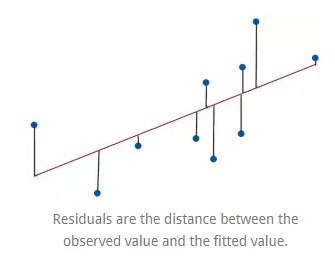
Statisticians say that a regression model fits the data well if the differences between the observations and the predicted values are small and biased. Unbiased in this context means that the fitted values are not systematically too high or too low anywhere in the observation space.

However, before assessing numeric measures of goodness-of-fit, like R-squared, we should evaluate the residual plots. Residual plots can expose a biased model far more effectively than the numeric output by displaying problematic patterns in the residuals.

R-squared and the Goodness-of-Fit

R-squared evaluates the scatter of the data points around the fitted regression line. It is also called the coefficient of determination, or the coefficient of multiple determination for multiple regression. For the same data set, higher R-squared values represent smaller differences between the observed data and the fitted values.

R-squared is the percentage of the dependent variable variation that a linear model explains.

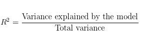
R-squared is always between 0 and 100%:

• 0% represents a model that does not explain any of the variations in the response variable around its mean. The mean of the dependent variable predicts the dependent variable as well as the regression model.
• 100% represents a model that explains all of the variations in the response variable around its mean.

Usually, the larger the R², the better the regression model fits your observations.

Visual Representation of R-square

To visually demonstrate how R-squared values represent the scatter around the regression line, we can plot the fitted values by observed values.

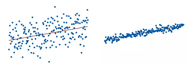
The R-squared for the regression model on the left is 15%, and for the model on the right, it is 85%. When a regression model accounts for more of the variance, the data points are closer to the regression line. In practice, we will never see a regression model with an R² of 100%. In that case, the fitted values equal the data values and, consequently, all of the observations fall exactly on the regression line.

R-square has Limitations

We cannot use R-squared to determine whether the coefficient estimates and predictions are biased, which is why you must assess the residual plots.

R-squared does not indicate if a regression model provides an adequate fit to your data. A good model can have a low R² value. On the other hand, a biased model can have a high R² value!

Are Low R-squared Values Always a Problem?

No. Regression models with low R-squared values can be perfectly good models for several reasons.

Some fields of study have an inherently greater amount of unexplainable variation. In these areas, your R² values are bound to be lower. For example, studies that try to explain human behavior generally have R² values of less than 50%. People are just harder to predict than things like physical processes.

Fortunately, if you have a low R-squared value but the independent variables are statistically significant, you can still draw important conclusions about the relationships between the variables. Statistically, significant coefficients continue to represent the mean change in the dependent variable given a one-unit shift in the independent variable.

There is a scenario where small R-squared values can cause problems. If we need to generate predictions that are relatively precise (narrow prediction intervals), a low R² can be a show stopper.

How high does R-squared need to be for the model produce useful predictions? That depends on the precision that you require and the amount of variation present in your data.

Are High R-squared Values Always Great?

No! A regression model with high R-squared value can have a multitude of problems. We probably expect that a high R² indicates a good model but examine the graphs below. The fitted line plot models the association between electron mobility and density.

The data in the fitted line plot follow a very low noise relationship, and the R-squared is 98.5%, which seems fantastic. However, the regression line consistently under and over-predicts the data along the curve, which is bias. The Residuals versus Fits plot emphasizes this unwanted pattern. An unbiased model has residuals that are randomly scattered around zero. Non-random residual patterns indicate a bad fit despite a high R².

This type of specification bias occurs when our linear model is underspecified. In other words, it is missing significant independent variables, polynomial terms, and interaction terms. To produce random residuals, try adding terms to the model or fitting a nonlinear model.

A variety of other circumstances can artificially inflate our R². These reasons include overfitting the model and data mining. Either of these can produce a model that looks like it provides an excellent fit to the data but in reality, the results can be entirely deceptive.

An overfit model is one where the model fits the random quirks of the sample. Data mining can take advantage of chance correlations. In either case, we can obtain a model with a high R² even for entirely random data!

R-squared Is Not Always Straightforward!

At first glance, R-squared seems like an easy to understand statistic that indicates how well a regression model fits a data set. However, it doesn’t tell us the entire story. To get the full picture, we must consider R² values in combination with residual plots, other statistics, and in-depth knowledge of the subject area.

Model Evaluation Metrics for Machine Learning

How to Interpret Adjusted R-Squared and Predicted R-Squared in Regression Analysis?

R-square tends to reward you for including too many independent variables in a regression model, and it doesn’t provide any incentive to stop adding more. Adjusted R-squared and predicted R-squared use different approaches to help you fight that impulse to add too many. The protection that adjusted R-squared and predicted R-squared provide is critical because too many terms in a model can produce results that we can’t trust.

Multiple Linear Regression can incredibly tempt statistical analysis that practically begs you to include additional independent variables in your model. Every time you add a variable, the R-squared increases, which tempts you to add more. Some of the independent variables will be statistically significant.

Some Problems with R-squared

We cannot use R-squared to conclude whether your model is biased.  To check for this bias, we need to check our residual plots. Unfortunately, there are yet more problems with R-squared that we need to address.

Problem 1: R-squared increases every time you add an independent variable to the model. The R-squared never decreases, not even when it’s just a chance correlation between variables. A regression model that contains more independent variables than another model can look like it provides a better fit merely because it contains more variables.

Problem 2: When a model contains an excessive number of independent variables and polynomial terms, it becomes overly customized to fit the peculiarities and random noise in our sample rather than reflecting the entire population.

Fortunately for us, adjusted R-squared and predicted R-squared address both of these problems.

Logistic Regression With Examples in Python and R