By: Prof. Mukesh Rao (Senior Faculty, Academics, Great Learning)
As a student of data science, one has likely encountered various statistical distributions, such as the Normal, Binomial, Multinomial, Chi-square, and T distributions, among others. What are these distributions, and why does a student of data science have to go through all this?
This post is based on a brief interaction with a beginner in data science who was attending a series of sessions in his course that covered these distributions and had no idea what was going on. The faculty presented these distributions without discussing the context, meaning, or application of these distributions. This is not uncommon.
Many students experience the same confusion while learning these topics, and this post aims to address those exact concerns. The concepts, meanings, and applications of these distributions are discussed here with the hope that they will help newcomers. Insights shared in this post are drawn from various online resources and practical experience in market research.
Let us start by understanding the concept of mathematical models, as distributions and mathematical models are two sides of the same coin.
The Role of Statistical Distributions
The first and foremost point a student of data science needs to understand and always keep in mind is that all the models built are representations of real-world processes. They mimic the behaviour of some real-world process. How well they do that depends on how well they were built. Why build such models? To predict the future behaviour of a process.
All statistical distributions are mathematical models representing the behaviour of consistent processes. They are models built by statisticians to represent process behaviour in various fields (sociology, biology, medicine, gaming, etc.).
These models are defined by their distribution characteristics, including central values, spread, shape (as measured by kurtosis and skewness), and others, as observed in the data generated by the processes under study.
To mathematically model the process of generating the data, a sample of data is drawn from the population. The sample may consist of all attributes or a subset of attributes, and all data points generated to date, or a subset of the data points. Usually, the larger the sample size in terms of the number of data points and the attributes, the better the model is likely to be.
The population, being dynamic, may also change in terms of the statistical distributions while work is being done on the sample data to build a model. These changes are unlikely to be significantly large unless a considerable amount of time is taken to develop and deploy the models. All models will gradually lose predictive power as the population characteristics change with time. This is called Concept Drift.
Hypothesis testing statistically helps assess the reliability of the sample data. Hypothesis testing compares the statistical distribution characteristics of two datasets (Population and Sample in this discussion) to determine their similarity.
Core Distributions Every Data Scientist Should Know
1. Normal Distribution
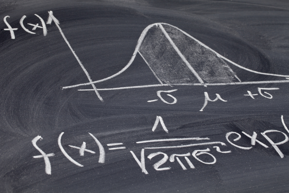
The normal distribution is a continuous probability distribution that is symmetrical around its mean. All three central values, i.e., the Mean, Median, and Mode, coincide. The variable values are symmetrically clustered around the central values.
Probability values can be extracted from the normal distribution, reflecting the capability of the process related to this distribution. For example, to estimate the probability of fixing tickets in the range V1 to V2 per day, find the area under the curve between V1 and V2 (Green area), and divide by the total area under the curve. That gives the required probability.
Unique characteristics of Normal distribution:
- The mean, median, and mode are all equal.
- The curve is symmetric around the mean.
- Exactly half of all the values are to the left of the centre, and half are to the right.
- The total area under the curve can be found using integral calculus.
- Empirical rule with 1 standard deviation (Standard Normal Distribution).
Concepts like Normal and Binomial distributions are core topics in industry-aligned programs such as the MS in Data Science Programme from Northwestern University, which blends theoretical rigour with practical exposure to tools like Python and R.
MS in Data Science Programme from Northwestern University
Advance your data science career with Northwestern’s globally recognized, 100% live online MS. Specialize in AI, complete in 18 months. Learn from world-class faculty.
2. Binomial Distribution
Suppose the process of filling packaged water bottles in a factory is being assessed. Every bottle that comes out of the process is supposed to contain 1 litre of water in volume. The focus is on how many bottles have failed to meet the standards on different attributes (defective).
Further, assume the output of this process is a carton of 11 filled bottles. If a carton is found to contain 6 or more defective bottles, the entire carton is rejected. Thus, to assess the process capability, the probability of six or more defective bottles in a carton needs to be found.
The term Binomial indicates two possible outcomes of an experiment (inspection of a bottle): either the bottle is good or it is bad.
Applications of Binomial probability:
- Probability of three or more servers in a rack going down at the same time.
- Helpful in designing technical architecture by evaluating failure scenarios.
3. Poisson Distribution
Poisson is a discrete probability distribution. This model represents processes that generate information in the form of counts, i.e., integer values. For example, the number of defects per unit output.
The Poisson distribution can be studied on a time axis, in space, or volume. In this example, the analysis is done on the time axis.
Given the average and variance, the probability of K events per interval can be found using the formula.
Applications of Poisson Distributions:
- Number of network intrusions per day
- Number of units likely to sell given average sales per unit time
- Number of website visitors per day
- Number of customer arrivals at a shop per day
- Number of calls per unit time at a call centre
For professionals who wish to explore advanced probabilistic models and their impact on decision-making systems, the Master of Data Science (Global) by Deakin University offers a strong foundation in both statistics and machine learning.
MIT Data Science and Machine Learning Course
Unlock the power of data. Build hands-on data science and machine learning skills to drive innovation in your career.
4. Chi-Square Distribution
Chi-squared distribution (also chi-square or χ²-distribution) with k degrees of freedom is the distribution of a sum of the squares of k independent standard normal random variables.
This means that any number of standard normal variables (K) can undergo the same transformations to result in a one-dimensional density plot.
As the value of K increases (i.e., degree of freedom), the composite density plot on one dimension tends to resemble the normal distribution.
Advantages of Chi-Square Analysis:
Thousands of variables with standard normal distribution can be represented by one single composite variable using the Chi-Square approach.
Uses of Chi-Square Distribution:
- Chi-squared tests for goodness of fit of an observed distribution to a theoretical one
- Testing independence of two classification criteria of qualitative data
- Confidence interval estimation for a population standard deviation from a sample standard deviation
Understanding statistical distributions is foundational for any data science journey. Whether evaluating the effectiveness of a production line, modelling customer behaviour, or ensuring data reliability, these distributions offer the mathematical lenses to interpret the real world. Start with a few Normal, Binomial, Poisson, and Chi-Square and explore others based on specific needs.
Each represents a consistent process and empowers the ability to predict and analyse with confidence.