- What are autoencoders
- Architecture of autoencoders
- Types of autoencoders
- Applications of autoencoders
- Implementation
What are Autoencoders
Autoencoder is a type of neural network where the output layer has the same dimensionality as the input layer. In simpler words, the number of output units in the output layer is equal to the number of input units in the input layer. An autoencoder replicates the data from the input to the output in an unsupervised manner and is therefore sometimes referred to as a replicator neural network.
The autoencoders reconstruct each dimension of the input by passing it through the network. It may seem trivial to use a neural network for the purpose of replicating the input, but during the replication process, the size of the input is reduced into its smaller representation. The middle layers of the neural network have a fewer number of units as compared to that of input or output layers. Therefore, the middle layers hold the reduced representation of the input. The output is reconstructed from this reduced representation of the input.
Architecture of autoencoders
An autoencoder consists of three components:
- Encoder: An encoder is a feedforward, fully connected neural network that compresses the input into a latent space representation and encodes the input image as a compressed representation in a reduced dimension. The compressed image is the distorted version of the original image.
- Code: This part of the network contains the reduced representation of the input that is fed into the decoder.
- Decoder: Decoder is also a feedforward network like the encoder and has a similar structure to the encoder. This network is responsible for reconstructing the input back to the original dimensions from the code.
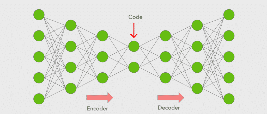
First, the input goes through the encoder where it is compressed and stored in the layer called Code, then the decoder decompresses the original input from the code. The main objective of the autoencoder is to get an output identical to the input.
Note that the decoder architecture is the mirror image of the encoder. This is not a requirement but it’s typically the case. The only requirement is the dimensionality of the input and output must be the same.
Types of autoencoders
There are many types of autoencoders and some of them are mentioned below with a brief description
Convolutional Autoencoder: Convolutional Autoencoders(CAE) learn to encode the input in a set of simple signals and then reconstruct the input from them. In addition, we can modify the geometry or generate the reflectance of the image by using CAE. In this type of autoencoder, encoder layers are known as convolution layers and decoder layers are also called deconvolution layers. The deconvolution side is also known as upsampling or transpose convolution.
Variational Autoencoders: This type of autoencoder can generate new images just like GANs. Variational autoencoder models tend to make strong assumptions related to the distribution of latent variables. They use a variational approach for latent representation learning, which results in an additional loss component and a specific estimator for the training algorithm called the Stochastic Gradient Variational Bayes estimator. The probability distribution of the latent vector of a variational autoencoder typically matches the training data much closer than a standard autoencoder. As VAEs are much more flexible and customisable in their generation behaviour than GANs, they are suitable for art generation of any kind.
Denoising autoencoders: Denoising autoencoders add some noise to the input image and learn to remove it. Thus avoiding to copy the input to the output without learning features about the data. These autoencoders take a partially corrupted input while training to recover the original undistorted input. The model learns a vector field for mapping the input data towards a lower-dimensional manifold which describes the natural data to cancel out the added noise. By this means, the encoder will extract the most important features and learn a more robust representation of the data.
Deep autoencoders: A deep autoencoder is composed of two symmetrical deep-belief networks having four to five shallow layers. One of the networks represents the encoding half of the net and the second network makes up the decoding half. They have more layers than a simple autoencoder and thus are able to learn more complex features. The layers are restricted Boltzmann machines, the building blocks of deep-belief networks.
Application of autoencoders
So far we have seen a variety of autoencoders and each of them is good at a specific task. Let’s find out some of the tasks they can do
Data Compression
Although autoencoders are designed for data compression yet they are hardly used for this purpose in practical situations. The reasons are:
- Lossy compression: The output of the autoencoder is not exactly the same as the input, it is a close but degraded representation. For lossless compression, they are not the way to go.
- Data-specific: Autoencoders are only able to meaningfully compress data similar to what they have been trained on. Since they learn features specific for the given training data, they are different from a standard data compression algorithm like jpeg or gzip. Hence, we can’t expect an autoencoder trained on handwritten digits to compress landscape photos.
Since we have more efficient and simple algorithms like jpeg, LZMA, LZSS(used in WinRAR in tandem with Huffman coding), autoencoders are not generally used for compression. Although autoencoders have seen their use for image denoising and dimensionality reduction in recent years.
Image Denoising
Autoencoders are very good at denoising images. When an image gets corrupted or there is a bit of noise in it, we call this image a noisy image.
To obtain proper information about the content of the image, we perform image denoising.
Dimensionality Reduction
“In statistics, machine learning, and information theory, dimensionality reduction, or dimension reduction is the process of reducing the number of random variables under consideration[1] by obtaining a set of principal variables. Approaches can be divided into feature selection and feature extraction.”
wikipedia
The autoencoders convert the input into a reduced representation which is stored in the middle layer called code. This is where the information from the input has been compressed and by extracting this layer from the model, each node can now be treated as a variable. Thus we can conclude that by trashing out the decoder part, an autoencoder can be used for dimensionality reduction with the output being the code layer.
Feature Extraction
Encoding part of Autoencoders helps to learn important hidden features present in the input data, in the process to reduce the reconstruction error. During encoding, a new set of combinations of original features is generated.
Image Generation
Variational Autoencoder(VAE) discussed above is a Generative Model, used to generate images that have not been seen by the model yet. The idea is that given input images like images of face or scenery, the system will generate similar images. The use is to:
- generate new characters of animation
- generate fake human images
Image colourisation
One of the applications of autoencoders is to convert a black and white picture into a coloured image. Or we can convert a coloured image into a grayscale image.
Implementations
In this section, we explore the concept of Image denoising which is one of the applications of autoencoders. After getting images of handwritten digits from the MNIST dataset, we add noise to the images and then try to reconstruct the original image out of the distorted image.
In this tutorial, we use convolutional autoencoders to reconstruct the image as they work better with images. Also, we use Python programming language along with Keras and TensorFlow to code this up.
from keras.datasets import mnist

### Importing Libraries

import keras
from keras import callbacks
from keras.models import Model
from keras.optimizers import Adadelta
from keras.layers import Input, Conv2D, MaxPool2D, UpSampling2D

### Downloading and Preprocessing of dataset and adding some noise to it.

import numpy as np

(trainX, trainy), (testX, testy) = mnist.load_data()

# to convert values from 0 to 255 into range 0 to 1.
trainX = np.expand_dims(trainX, axis=-1)
testX = np.expand_dims(testX, axis=-1)
trainX = trainX.astype("float32") / 255.0
testX = testX.astype("float32") / 255.0
The next step is to add noise to our dataset. For this purpose, we use the NumPy library to generate random numbers with a mean of 0.5 and a standard deviation of 0.5 in the shape of our input data. Also to make sure the values of a pixel in between 0 and 1, we use the clip function of NumPy to do so
#add noise to the images
trainNoise = np.random.normal(loc=0.5, scale=0.5, size=trainX.shape)
testNoise = np.random.normal(loc=0.5, scale=0.5, size=testX.shape)
trainXNoisy = np.clip(trainX + trainNoise, 0, 1)
testXNoisy = np.clip(testX + testNoise, 0, 1)
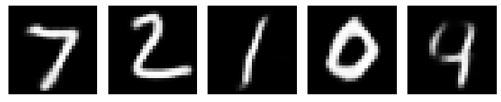
Now let us visualize the distorted dataset and compare it with our original dataset. Here I have displayed the five images before and after adding noise to them
import matplotlib.pyplot as plt
plt.figure(figsize=(10, 10))
for i in range(5):
  plt.subplot(1, 5, i+1)
  plt.xticks([])
  plt.yticks([])
  plt.grid(False)
  plt.imshow(trainX[i].reshape(28, 28), cmap='gray')
plt.tight_layout()
plt.show()

plt.figure(figsize=(10, 10))
for i in range(5):
  plt.subplot(1, 5, i+1)
  plt.xticks([])
  plt.yticks([])
  plt.grid(False)
  plt.imshow(trainXNoisy[i].reshape(28, 28), cmap='gray')
plt.tight_layout()
plt.show()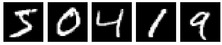
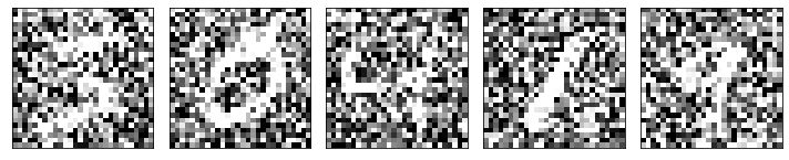
As we can see above, the images are partially distorted after adding noise to them and we can hardly recognize the digits. Next, we define the structure of our autoencoder, fit the distorted images, and pass the original images as labels.
input_img = Input(shape=(28, 28, 1)) # adapt this if using `channels_first` image data format
x = Conv2D(32, (3, 3), activation='relu', padding='same')(input_img)
x = MaxPool2D((2, 2), padding='same')(x)
x = Conv2D(32, (3, 3), activation='relu', padding='same')(x)
encoded = MaxPool2D((2, 2), padding='same')(x)
# at this point the representation is (7, 7, 32)
x = Conv2D(32, (3, 3), activation='relu', padding='same')(encoded)
x = UpSampling2D((2, 2))(x)
x = Conv2D(32, (3, 3), activation='relu', padding='same')(x)
x = UpSampling2D((2, 2))(x)
decoded = Conv2D(1, (3, 3), activation='sigmoid', padding='same')(x)
autoencoder = Model(input_img, decoded)
autoencoder.compile(optimizer='adadelta', loss='binary_crossentropy')
# train the convolutional autoencoder
H = autoencoder.fit(
trainXNoisy, trainX,
validation_data=(testXNoisy, testX),
epochs=20,
batch_size=32)
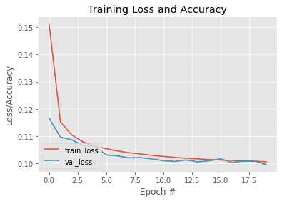
N = np.arange(0, 20)
plt.style.use("ggplot")
plt.figure()
plt.plot(N, H.history["loss"], label="train_loss")
plt.plot(N, H.history["val_loss"], label="val_loss")
plt.title("Training Loss and Accuracy")
plt.xlabel("Epoch #")
plt.ylabel("Loss/Accuracy")
plt.legend(loc="lower left")
plt.show()Output: Here is a plot which shows loss at each epoch for both training and validation sets
# predict the reconstructed images for the original images
pred = autoencoder.predict(testXNoisy)
## Visualizing our results
plt.figure(figsize=(10,10))
for i in range(5):
plt.subplot(1, 5, i+1)
plt.xticks([]) # to remove x-axis the [] empty list indicates this
plt.yticks([]) # to remove y-axis
plt.grid(False) # to remove grid
plt.imshow(testX[i].reshape(28, 28), cmap='gray') #display the image
plt.tight_layout() # to have a proper space in the subplots
plt.show()
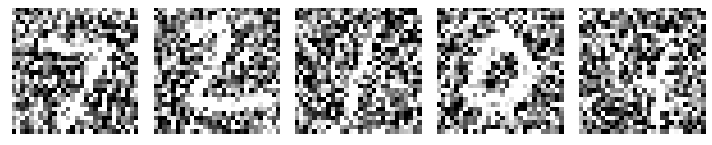
plt.figure(figsize=(10,10))
for i in range(5):
plt.subplot(1, 5, i+1)
plt.xticks([]) # to remove x-axis the [] empty list indicates this
plt.yticks([]) # to remove y-axis
plt.grid(False) # to remove grid
plt.imshow(testXNoisy[i].reshape(28, 28), cmap='gray') #display the image
plt.tight_layout() # to have a proper space in the subplots
plt.show()
# to visualise reconstructed images(output of autoencoder)
plt.figure(figsize=(10,10))
for i in range(5):
plt.subplot(1, 5, i+1)
plt.xticks([]) # to remove x-axis the [] empty list indicates this
plt.yticks([]) # to remove y-axis
plt.grid(False) # to remove grid
plt.imshow(pred[i].reshape(28, 28), cmap='gray') #display the image
plt.tight_layout() # to have a proper space in the subplots
plt.show()
As we can see above, the model is able to successfully denoise the images and generate the pictures that are pretty much identical to the original images
This brings us to the end of this article where we have learned about autoencoders in deep learning and how it can be used for image denoising.
If you wish to learn more about Python and the concepts of Machine Learning, upskill with Great Learning’s PG Program Artificial Intelligence and Machine Learning.