Supervised vs Unsupervised Learning
In Supervised Learning, we train the machine using data that is well "labeled". It means the data is already tagged with the correct answer. A supervised learning algorithm learns from labeled training data and predicts outcomes for unforeseen data. There are two subcategories of supervised learning, viz- Regression and Classification.
Classification means to group the output into a class. If the algorithm tries to label input into two distinct classes, it is called binary classification. Selecting between more than two classes is referred to as multiclass classification. On the other hand, Regression Algorithms are used to predict continuous values such as price, salary, and age.
Unsupervised Learning is a machine learning technique, where the model does not need any supervision. Instead, we need to allow the model to work on its own to discover information. It mainly deals with the unlabelled data. Density estimation, dimensionality reduction, and clustering and some of the main applications of unsupervised learning.
What are Generative Models?
The learning models in machine learning can be classified into two sub-categories, viz - Discriminative models and Generative models. To understand GANs, we should know about generative models and how they are different from Discriminative models.
Discriminative models classify input data; i.e., given the features of an instance of data, they predict a label or category to which that data belongs. In Supervised Learning, the classification algorithms/models are examples of discriminative models.
Generative Modelling is an unsupervised learning task in machine learning that involves generating new data samples from the probability distribution of training data. Given some data, the aim is to have a model for the underlying probability distribution of that data so that we can draw samples that are similar to our training data.
Mathematically, generative models learn the joint probability distribution P(X,Y), whereas the discriminative models learn the posterior probability, P(Y|X), that is the probability of the label Y given the data X.
Uses of Generative Models
1. It can help in generating artificial faces.
2. It can be used in Text to image generation.
3. It can produce fake voices or noises and can be used in image denoising.
4. It can be used in MRI image reconstruction.
5. It can also be used to generate instances of data to handle imbalanced data.
Generative models target the true distribution of the training data to generate new data points with some variations. Now, it is not always possible for our machine to learn the true distribution of the data, for this, we take the help of a powerful neural network which can help make the machine learn the approximate true distribution of the data.
The neural networks we use as generative models have parameters which are smaller than the amount of data we have as training dataset. The models are forced to discover the distribution in order to generate data.
PG Program in AI & Machine Learning
Master AI with hands-on projects, expert mentorship, and a prestigious certificate from UT Austin and Great Lakes Executive Learning.
What are GANs
Generative adversarial networks, also known as GANs are deep generative models and like most generative models they use a differential function represented by a neural network known as a Generator network. GANs also consist of another neural network called Discriminator network.
A Generator network takes random noise as input and runs that noise through the differential function to transform the noise and reshape it to get a recognisable structure. The output of the generator seems like a real data point. The choice of the random input voice determines which data point will come out of the generator network. Running the generator network with many different input noise values produces many different realistic output data samples. The goal for these generated data samples is to be the fair samples from the distribution of real data.
But the generator network needs to be trained before it can generate realistic data points as output. The training process for a generative model is different from that of the training process of a supervised model. For a supervised learning model, each input data is associated with its respective label whereas, for a generative model, the model is shown a lot of data samples and it makes new data samples that come from the same probability distribution.
GANs use an approximation where a second network called the Discriminator guides the Generator to generate the samples from the probability distribution of given data. The Discriminator is a regular neural network classifier that classifies the real samples from the fake samples generated by the Generator.
During the training process, the Discriminator is shown real samples half of the time and fake samples from the Generator the other half of the time. It assigns a probability close to ‘1’ to real samples and the probability close to ‘0’ to fake samples.
Meanwhile, the Generator is trying to output samples that the Discriminator would assign a probability of near one and classify them as real samples. Over time the generator is forced to produce the samples that are more realistic outputs in order to fool the Discriminator. It is clear that the two networks are competing against each other and can be termed as adversarial networks.
Note that this adversarial framework has transformed an unsupervised problem with raw data and no samples into a supervised problem with labels we create, that is, real and fake.
In the figure above, the blue line represents the distribution of Discriminator, the green line represents Generative distribution while the bell is the distribution of real data.
The Generator takes random noise value z and maps them to output values x. The probability distribution over x represented by the model becomes denser wherever more values of z are mapped. The Discriminator outputs high values wherever the density of real data is greater than the density of generated data. The Generator changes the samples it produces to move uphill along the function learned by the Discriminator and eventually the Generator’s distribution matches the distribution of real data. Due to this, the Discriminator outputs the probability of 0.5 for every sample because every sample is equally likely to be generated by the real data-set as it is to be generated by the Generator.
We can think of this process as a competition between police and counterfeiters. The Generator network is like a counterfeiter trying to produce fake money and pass it off as real. The police act as a Discriminator network and want to catch the counterfeiter spending the fake money but also do not want to stop people using real money. Over time the police get better at recognising fake money but at the same time, the counterfeiter also improves his techniques to produce fake currency. At some point, the counterfeiter makes exact replicas of the currency and the police can no longer discriminate between the real and fake money.
Where are GANs used
Most of the applications for GANs have been in the field of computer vision. More specifically GANs are good at generating images that have never been seen before. Some of the models that have used GANs are described below:
- StackGAN model: StackGAN model is good at generating images from the description. Text to image synthesis is one of the use cases for Generative Adversarial Networks (GANs) that has many industrial applications. Synthesizing images from text descriptions is a very hard task, as it is very difficult to build a model that can generate images that reflect the meaning of the text.
- pix2pix model: pix2pix are used for image translation which means that images in one domain can be transformed into images of another domain, For example, blueprints of a building can be transformed into photos of the finished building, or drawing of cats can be transformed into real images of cats
- CycleGAN: CycleGAN is an unsupervised approach to training image-to-image translation models using the generative adversarial network, or GAN, model architecture. Some of the popular applications of CycleGANs are Object Transfiguration, For example changing an image of horses into zebras or vice-versa.
Post Graduate Program in Generative AI for Business Applications
Discover the power of generative AI in real-world business scenarios. Learn to lead with data-driven insights and strategy.
Tips for Training GANs
To make GANs work well, it is essential to choose a good architecture. For simple tasks like generating 28 x 28 images of handwritten digits of the MNIST dataset, we can use a fully connected architecture. In this type of architecture, we do not use any convolutional or recurrent layers.
Both the Generator as well as Discriminator must have at least one hidden layer to ensure that they can represent any probability distribution. For the hidden layers, we use “LeakyRELU” as the activation function as they make sure that the gradient can flow through the entire architecture.
A popular choice for the output of the Generator is to use “tanh” (hyperbolic tan) activation function which ensures that the data is in the interval between -1 to +1. The output of discriminator needs to be a probability, to force this constraint we use the sigmoid unit as the output.
Generating MNIST Handwritten Digit
In this section, we are going to use a fully connected architecture of GANs to generate MNIST handwritten digits. We use Python programming language along with Keras library for implementation.
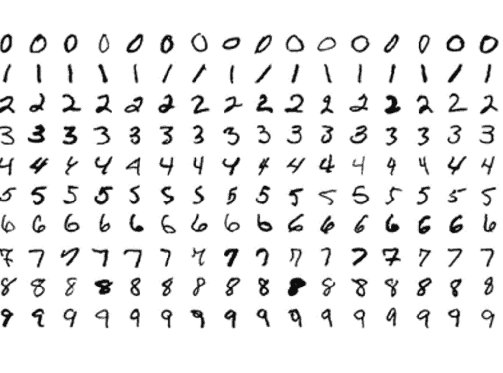
The MNIST dataset is an acronym that stands for the Modified National Institute of Standards and Technology dataset. It is a dataset of 70,000 small square 28×28 pixel grayscale images of handwritten single digits between 0 and 9.
 # example of training a gan on mnist
 # import all necessary libararies
  from numpy import expand_dims
  from numpy import zeros
  from numpy import ones
  from numpy import vstack
  from numpy.random import randn
  from numpy.random import randint
  from keras.datasets.mnist import load_data
  from keras.optimizers import Adam
  from keras.models import Sequential
  from keras.layers import Dense
  from keras.layers import Reshape
  from keras.layers import Flatten
  from keras.layers import Conv2D
  from keras.layers import Conv2DTranspose
  from keras.layers import LeakyReLU
  from keras.layers import Dropout
  from matplotlib import pyplot

  # define the standalone discriminator model
  def define_discriminator():
    d = Sequential()
  # input_dim is modified from 28x28 to 784
    d.add(Dense(1024, input_dim=784, activation=LeakyReLU(alpha=0.2)))
    d.add(Dropout(0.3))
    d.add(Dense(512, activation=LeakyReLU(alpha=0.2)))
    d.add(Dropout(0.3))
    d.add(Dense(256, activation=LeakyReLU(alpha=0.2)))
    d.add(Dropout(0.3))
    d.add(Dense(1, activation='sigmoid'))  # Values between 0 and 1
    d.compile(loss='binary_crossentropy', optimizer=Adam(lr=0.0002, beta_1=0.5), metrics=['accuracy'])
    return d


  # define the standalone generator model
  def define_generator(latent_dim):
    g = Sequential()
#latent_dim is dimnetion of noise.It can be anything like 10,50,100
    g.add(Dense(256, input_dim=latent_dim, activation=LeakyReLU(alpha=0.2)))
    g.add(Dense(512, activation=LeakyReLU(alpha=0.2)))
    g.add(Dense(1024, activation=LeakyReLU(alpha=0.2)))
    g.add(Dense(784, activation='tanh'))  # Values between -1 and 1
    g.compile(loss='binary_crossentropy', optimizer=Adam(lr=0.0002, beta_1=0.5), metrics=['accuracy'])
    return g


  # define the combined generator and discriminator model, for updating the generator
  def define_gan(g_model, d_model):
    # make weights in the discriminator not trainable
    #so that it doesnt change when training generator
    d_model.trainable = False
    # connect them
    model = Sequential()
    # add generator
    model.add(g_model)
    # add the discriminator
    model.add(d_model)
    # compile model
    opt = Adam(lr=0.0002, beta_1=0.5)
    model.compile(loss='binary_crossentropy', optimizer=opt)
    return model

  # load and prepare mnist training images
  def load_real_samples():
    # load mnist dataset
    (trainX, _), (_, _) = load_data()
    # expand to 3d, e.g. add channels dimension
    X = trainX.reshape(60000, 784)
    # convert from unsigned ints to floats
    X = X.astype('float32')
    # scale from [0,255] to [0,1]
    X = X / 255.0
    return X

  # select real samples
  def generate_real_samples(dataset, n_samples):
    # choose random instances
    ix = randint(0, dataset.shape[0], n_samples)
    # retrieve selected images
    X = dataset[ix]
    # generate 'real' class labels (1)
    y = ones((n_samples, 1))
    return X, y

  # generate points in latent space as input for the generator
  def generate_latent_points(latent_dim, n_samples):
    # generate points in the latent space
    x_input = randn(latent_dim * n_samples)
    # reshape into a batch of inputs for the network
    x_input = x_input.reshape(n_samples, latent_dim)
    return x_input

  # use the generator to generate n fake examples, with class labels
  def generate_fake_samples(g_model, latent_dim, n_samples):
    # generate points in latent space
    x_input = generate_latent_points(latent_dim, n_samples)
    # predict outputs
    X = g_model.predict(x_input)
    # create 'fake' class labels (0)
    y = zeros((n_samples, 1))
    return X, y


  def plot_loss(losses):

      d_loss = [v for v in losses["D"]]
      g_loss = [v for v in losses["G"]]

      plt.figure(figsize=(10,8))
      plt.plot(d_loss, label="Discriminator loss")
      plt.plot(g_loss, label="Generator loss")

      plt.xlabel('Epochs')
      plt.ylabel('Loss')
      plt.legend()
      plt.show()

  def plot_generated(n_ex=10, dim=(1, 10), figsize=(12, 2)):
      noise = np.random.normal(0, 1, size=(n_ex, z_dim))
      generated_images = g_model.predict(noise)
      generated_images = generated_images.reshape(generated_images.shape[0], 28, 28)
      plt.figure(figsize=figsize)
      for i in range(generated_images.shape[0]):
          plt.subplot(dim[0], dim[1], i+1)
          plt.imshow(generated_images[i, :, :], interpolation='nearest', cmap='gray_r')
          plt.axis('off')
      plt.tight_layout()
      plt.show()

  # train the generator and discriminator
  def train(g_model, d_model, gan_model, dataset, latent_dim, n_epochs=100, n_batch=256):
    losses = {"D":[], "G":[]}
    samples = []
    bat_per_epo = int(dataset.shape[0] / n_batch)
    half_batch = int(n_batch / 2)
    # manually enumerate epochs
    for i in range(n_epochs):
      # enumerate batches over the training set
      for j in range(bat_per_epo):
        # get randomly selected 'real' samples
        X_real, y_real = generate_real_samples(dataset, half_batch)
        # generate 'fake' examples
        X_fake, y_fake = generate_fake_samples(g_model, latent_dim, half_batch)
        # create training set for the discriminator
        X, y = vstack((X_real, X_fake)), vstack((y_real, y_fake))
        # update discriminator model weights
        d_model.trainable = True
        d_loss, _ = d_model.train_on_batch(X, y)
        # prepare points in latent space as input for the generator
        X_gan = generate_latent_points(latent_dim, n_batch)
        # create inverted labels for the fake samples
        y_gan = ones((n_batch, 1))
        # update the generator via the discriminator's error
        d_model.trainable = False #discriminator is not trained while training gan
        g_loss = gan_model.train_on_batch(X_gan, y_gan)
      print("###################### epoch {} completed #########################".format(i))
      plot_generated()
      # Only store losses from final batch of epoch
      losses["D"].append(d_loss)
      losses["G"].append(g_loss)
     # Update the plots
    plot_loss(losses)


  # size of the latent space
  latent_dim = 100
  # create the discriminator
  d_model = define_discriminator()
  # create the generator
  g_model = define_generator(latent_dim)
  # create the gan
  gan_model = define_gan(g_model, d_model)
  # load image data
  dataset = load_real_samples()
  # train model
  train(g_model, d_model, gan_model, dataset, latent_dim,n_epochs=200)
Output:
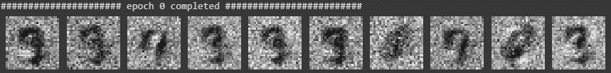
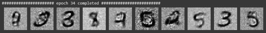
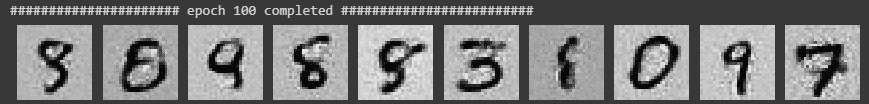
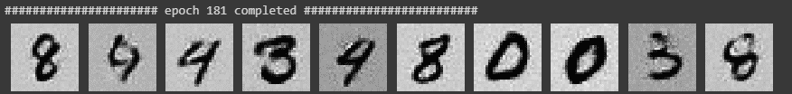
As we can see we are able to generate decent replicas of the MNIST dataset. Although an alternative is to use DCGANs (Deep Convolutional GANs) which may produce better results than a simple MPL (Multi-Layered Perceptron) which we used here.
Variational Autoencoders(VAE)
VAE are deep latent variables (Latent variables are the variables which we cannot observe in training and test datasets. These variables cannot be measured on a quantitative scale) models that use artificial neural networks to infer an approximate posterior over latent variables and to generate new data samples.
VAE are deep learning techniques which are recognized as being able to draw images, interpolate between sentences and achieve great results in semi supervised learning.
This brings us to the end of this article where we have learned about GANs in deep learning and its implementation.
If you wish to learn more about Python and the concepts of ML, upskill with Great Learning’s PG Program Artificial Intelligence and Machine Learning.