Data Preprocessing for Machine Learning – Step-by-Step Guide

You have a dataset and a goal. Between them lies the most critical and time-consuming phase of any machine learning project: data preprocessing.

Feeding raw, messy data directly into an algorithm is a guaranteed path to failure. The quality of your model is not determined by the complexity of the algorithm you choose, but by the quality of the data you feed it.

This guide is a step-by-step breakdown of the essential preprocessing tasks. We will not waste time on abstract theory. Instead, we will focus on the practical sequence of operations you must perform to transform chaotic, real-world data into a clean, structured format that gives your model its best chance at success.

Step 1: First Thing to Do – Split Your Data

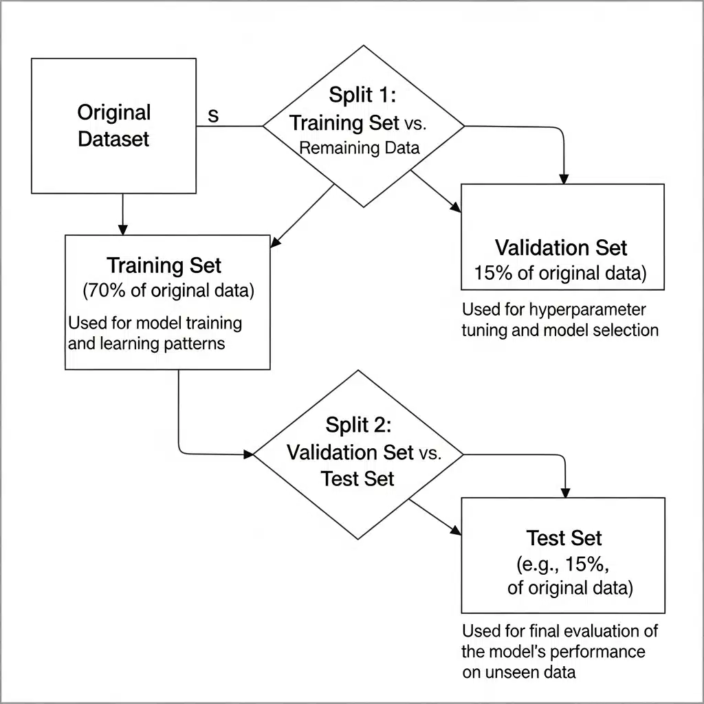
Before you touch, clean, or even look at your data too closely, split it. You need separate training, validation, and testing sets.

• Training Set: The bulk of your data. The model learns from this.
• Validation Set: Used to tune your model’s hyperparameters and make decisions during training. It’s a proxy for unseen data.
• Test Set: Kept in a vault, untouched until the very end. This is for the final, unbiased evaluation of your trained model.

Why split first?

To prevent data leakage. Data leakage is when information from outside the training dataset is used to create the model. If you calculate the mean of a feature using the entire dataset and then use that to fill missing values in your training set, your model has already “seen” the test data. Its performance will be artificially inflated, and it will fail in the real world.

Split first, then do all your preprocessing calculations (like finding the mean, min, max, etc.) only on the training set. Then, apply those same transformations to the validation and test sets.

A common split is 70% for training, 15% for validation, and 15% for testing, but this can change. For huge datasets, you might use a 98/1/1 split because 1% is still a statistically significant number of samples. For time-series data, you don’t split randomly. Your test set should always be “in the future” relative to your training data to simulate a real-world scenario.

Step 2: Data Cleaning

Real-world data is messy. It has missing values, outliers, and incorrect entries. Your job is to clean it up.

Handling Missing Values

Most machine learning algorithms can’t handle missing data. You have a few options, and “just drop it” isn’t always the best one.

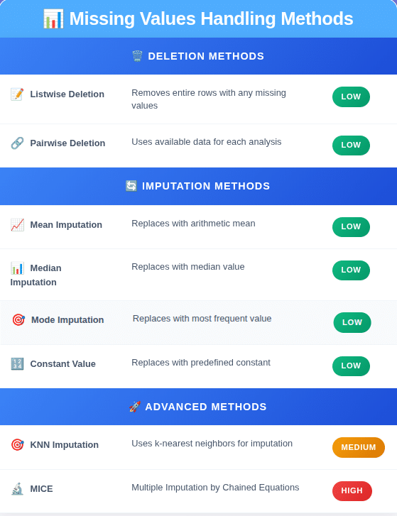
Deletion:

• Listwise Deletion (Drop Rows): If a row has one or more missing values, you delete the entire row. This is simple but risky. If you have a lot of missing data, you could end up throwing away a huge chunk of your dataset.
• Pairwise Deletion (Drop Columns): If a column (feature) has a high percentage of missing values (e.g., > 60-70%), it might be useless. Deleting the entire column can be a valid strategy.

Imputation (Filling in Values):

This is usually the better approach, but you have to be careful.

• Mean/Median/Mode Imputation: Replace missing numerical values with the mean or median of the column. Use the median if the data has a lot of outliers, as the mean is sensitive to them. For categorical features, use the mode (the most frequent value). This is a basic approach and can reduce variance in your data.
• Constant Value Imputation: Sometimes a missing value has a meaning. For example, a missing Garage_Finish_Date might mean the house has no garage. In this case, you can fill the missing values with a constant like “None” or 0. For numerical features, you could impute with a value far outside the normal range, like -1, to let the model know it was originally missing.
• Advanced Imputation (KNN, MICE): More complex methods use other features to predict the missing values. K-Nearest Neighbors (KNN) imputation finds the ‘k’ most similar data points and uses their values to impute the missing one. Multiple Imputation by Chained Equations (MICE) is a more robust method that creates multiple imputed datasets and pools the results. These are computationally more expensive but often more accurate.

A good practice is to create a new binary feature that indicates whether a value was imputed. For a feature age, you would create age_was_missing. This lets the model learn if the fact that the data was missing is itself a predictive signal.

Step 3: Handling Categorical Data

Models understand numbers, not text. You need to convert categorical data like “Color” or “City” into a numerical format.

Label Encoding

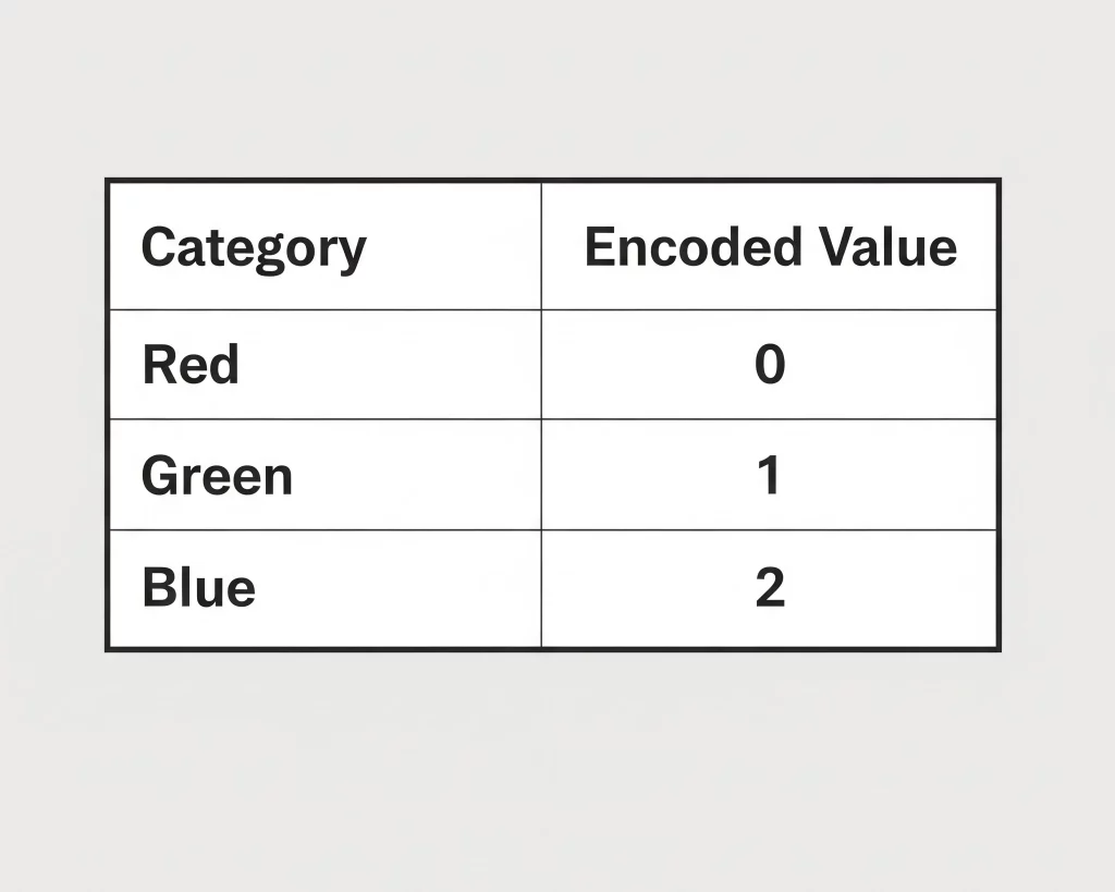
• What it is: Assigns a unique integer to each category. Example: {‘Red’: 0, ‘Green’: 1, ‘Blue’: 2}.
• When to use it: Only for ordinal variables, where the categories have a meaningful order. For example, {‘Low’: 0, ‘Medium’: 1, ‘High’: 2}.
• When NOT to use it: For nominal variables where there is no intrinsic order, like colors or cities. Using it here introduces an artificial relationship; the model might think Blue (2) is “greater” than Green (1), which is meaningless and will hurt performance.

One-Hot Encoding

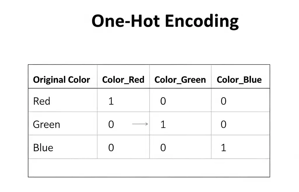
• What it is: Creates a new binary (0 or 1) column for each category. If the original feature was “Color” with categories Red, Green, and Blue, you get three new columns: Color_Red, Color_Green, and Color_Blue. For a “Red” data point, Color_Red would be 1, and the other two would be 0.
• When to use it: This is the standard approach for nominal categorical data. It removes the ordinal relationship problem.
• The Downside (Curse of Dimensionality): If a feature has many categories (e.g., 100 different cities), one-hot encoding will create 100 new columns. This can make your dataset huge and sparse, a problem known as the “curse of dimensionality,” which can make it harder for some algorithms to perform well.

Other Encoding Methods

For high-cardinality features (many categories), you can consider:

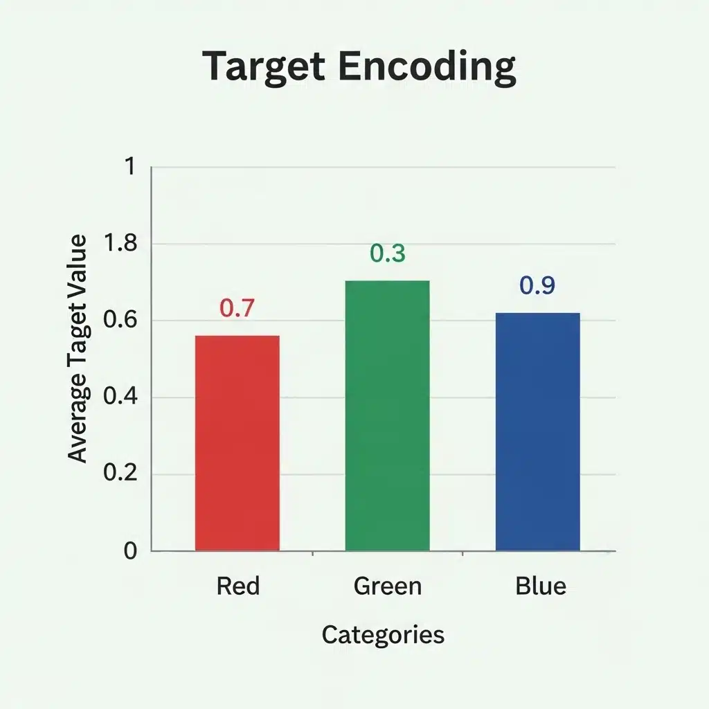
• Target Encoding: Replaces each category with the average value of the target variable for that category. This is powerful but has a high risk of overfitting, so it needs to be implemented carefully (e.g., using cross-validation).
• Feature Hashing (The “Hashing Trick”): Uses a hash function to map a potentially large number of categories to a smaller, fixed number of features. It’s memory-efficient but can have hash collisions (different categories mapping to the same hash).

Step 4: Feature Scaling – Putting Everything on the Same Level

Algorithms that use distance calculations (like KNN, SVM, and PCA) or gradient descent (like linear regression and neural networks) are sensitive to the scale of features. If one feature ranges from 0-1 and another from 0-100,000, the latter will dominate the model. You need to bring all features to a comparable scale.

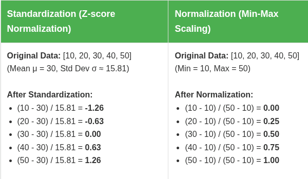
Standardization (Z-score Normalization)

• What it does: Transforms the data to have a mean of 0 and a standard deviation of 1. The formula is (x – mean) / std_dev.
• When to use it: This is the go-to method for many algorithms, especially when your data is roughly normally distributed. It doesn’t bind values to a specific range, which makes it less sensitive to outliers. PCA, for example, often requires standardization.

Normalization (Min-Max Scaling)

• What it does: Rescales the data to a fixed range, usually 0 to 1. The formula is (x – min) / (max – min).
• When to use it: Good for algorithms that don’t assume any distribution, like neural networks, as it can help with faster convergence. However, it’s very sensitive to outliers. A single extreme value can squash all the other data points into a very small range.
• Which one to choose? There’s no single right answer. Standardization is generally a safer default choice. If you have a reason to bound your data or your algorithm requires it, use normalization. When in doubt, you can always try both and see which performs better on your validation set. Tree-based models like Decision Trees and Random Forests are not sensitive to feature scaling.

Read in Detail: Data Normalization and Standardization

Step 5: Feature Engineering – Creating New Information

This is where domain knowledge and creativity come in. It’s the process of creating new features from existing ones to help your model learn better.

• Interaction Features: Combine two or more features. For example, if you have Height and Weight, you can create a BMI feature (Weight / Height^2). You might find that the interaction between Temperature and Humidity is more predictive of sales than either feature alone.
• Polynomial Features: Create new features by raising existing features to a power (e.g., age^2, age^3). This can help linear models capture non-linear relationships.
• Time-Based Features: If you have a datetime column, don’t just leave it. Extract useful information like hour_of_day, day_of_week, month, or is_weekend. For cyclical features like hour_of_day, simply using the number isn’t ideal because hour 23 is close to hour 0. A better approach is to use sine and cosine transformations to represent the cyclical nature.
• Binning: Convert a continuous numerical feature into a categorical one. For example, you can convert age into categories like 0-18, 19-35, 36-60, and 60+. This can sometimes help the model learn patterns in specific ranges.

Feature engineering is often an iterative process. You create features, train a model, analyze the results, and then go back to create more informed features.

Final Word

Data preprocessing is not a rigid checklist; it’s a thoughtful process that depends heavily on your specific dataset and the problem you’re trying to solve. Always document the steps you take and the reasons for your decisions. This makes your work reproducible and easier to debug when your model inevitably does something unexpected. Good preprocessing is the foundation of a good model.