- What is Support Vector Machine (SVM)?
- Support Vector Machine (SVM) Visualization
- How Does SVM Classify Data?
- Mathematical Foundation of SVM Algorithm
- Types of SVM
- The Kernel Trick: Handling Non-Linearity
- Real-World Applications of SVM
- Support Vector Machine Example: Solving a Classification Problem
- Conclusion
- Frequently Asked Questions
Support Vector Machine (SVM) is a supervised machine learning algorithm used for classification and regression tasks. It is widely applied in fields like image recognition, text classification, and bioinformatics due to its efficiency in handling high-dimensional data.
In this article, we will start from the basics of SVM in machine learning, gradually diving into its working principles, different types, mathematical formulation, real-world applications, and implementation.
What is Support Vector Machine (SVM)?
SVM is a classification algorithm that finds the best boundary (hyperplane) to separate different classes in a dataset. It works by identifying key data points, called support vectors, that influence the position of this boundary, ensuring maximum separation between categories.
For example, if we have a dataset of emails labeled as spam and not spam, SVM will create a decision boundary that best separates these two groups based on features like word frequency and message length.
Support Vector Machine (SVM) Visualization
What SVM Does:
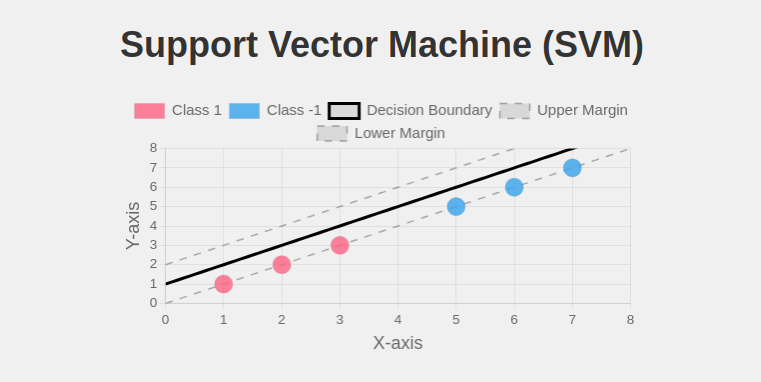
Support Vector Machines (SVM) find the optimal hyperplane that maximizes the margin between two classes. The margin is the distance between the decision boundary and the closest data points from each class, which are called support vectors.
In this visualization:
- The black line represents the decision boundary
- The dashed lines represent the margins
- Highlighted points are support vectors
- Red and teal dots represent different classes
SVM aims to find the hyperplane that has the maximum margin, as this typically leads to better generalization on unseen data.
How Does SVM Classify Data?
SVM follows these steps to classify data:
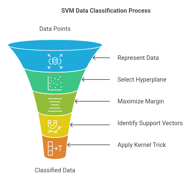
- Data Representation: Each data point is represented as a vector in an n-dimensional space.
- Hyperplane Selection: SVM finds the optimal hyperplane that separates the data into distinct classes.
- Maximizing the Margin: It ensures that the separation margin between classes is as wide as possible to improve generalization.
- Using Support Vectors: The closest points to the hyperplane (support vectors) influence its placement.
- Kernel Trick (for Non-Linearity): If the data is not linearly separable, SVM transforms it into a higher dimension using kernel functions.
Also Read: Support Vector Regression in Machine Learning
Mathematical Foundation of SVM Algorithm
For two-class classification, given a dataset (xi, yi), where xi are feature vectors and yi are class labels (either +1 or -1), SVM aims to minimize the function:
minw,b (1/2) ||w||2
Subject to:
yi (w · xi + b) ≥ 1 for all i
where:
- w represents the weight vector,
- b is the bias term,
- ||w||2 ensures the maximization of the margin.
In cases where data points are not entirely separable, slack variables ξ are introduced, modifying the function as follows:
minw,b,ξ (1/2) ||w||2 + C Σ ξi
Here, C controls the trade-off between maximizing the margin and minimizing classification errors.
Types of SVM
SVM can be classified into different types based on the nature of the dataset:
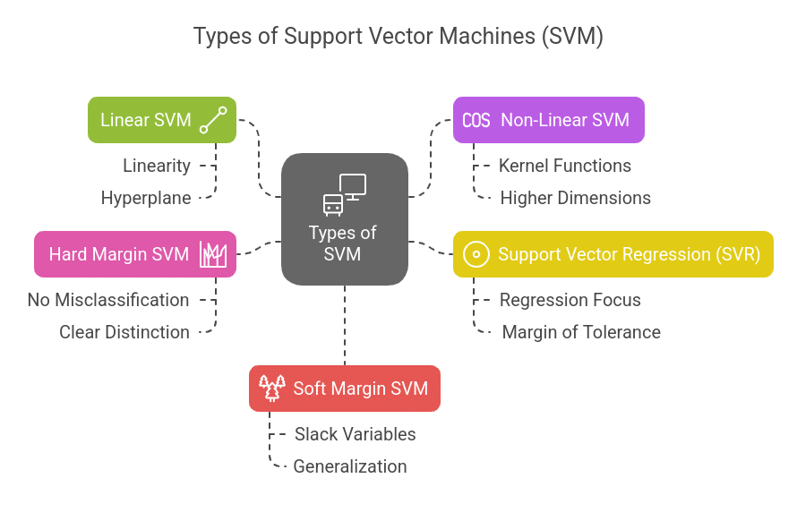
- Linear SVM: Used when data can be separated using a straight hyperplane. It is suitable for datasets where classes are linearly separable. The decision boundary is a straight line (in 2D) or a plane (in higher dimensions).
- Non-Linear SVM: When data is not linearly separable, kernel functions are used to map data into a higher-dimensional space where separation is possible. Kernel functions like RBF and polynomials are commonly used in non-linear SVM.
- Support Vector Regression (SVR): A variation of SVM used for regression problems instead of classification. It works similarly to classification SVM but tries to fit a function within a margin of tolerance rather than finding a strict boundary between categories.
- Hard Margin SVM: Assumes that the data is perfectly separable and aims to find a hyperplane that classifies all data points correctly with no tolerance for misclassification. This works well when there is a clear distinction between classes.
- Soft Margin SVM: Introduces slack variables to handle cases where classes may overlap slightly. It allows some misclassifications to improve generalization and prevent overfitting.
The Kernel Trick: Handling Non-Linearity
Real-world data is often non-linearly separable. SVM uses kernel functions to transform data into a higher-dimensional space where it becomes separable. Some popular kernels include:
- Linear Kernel: K(x, y) = x · y (used in linear support vector machine)
- Polynomial Kernel: K(x, y) = (x · y + c)d
- Radial Basis Function (RBF) Kernel: K(x, y) = e−γ||x − y||2
Real-World Applications of SVM
SVM has practical use cases across different domains:
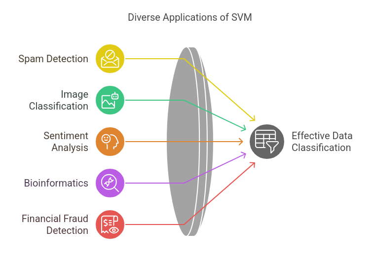
- Spam Detection: In this, we classify emails as spam or not spam.
- Image Classification: Recognizing objects, faces, or handwritten digits.
- Sentiment Analysis: Determining if a review is positive or negative.
- Bioinformatics: Identifying diseases based on genetic data.
- Financial Fraud Detection: Identifying unusual transaction patterns.
Discover the various Machine Learning Models and their role in predictions, classifications, and data-driven decision-making across industries.
Support Vector Machine Example: Solving a Classification Problem
Problem Statement:
A company wants to classify emails as spam or not spam based on features such as word frequency and message length.
Implementation:
import numpy as np
import pandas as pd
from sklearn.model_selection import train_test_split
from sklearn.feature_extraction.text import TfidfVectorizer
from sklearn.svm import SVC
from sklearn.metrics import accuracy_score, classification_report

# Sample dataset (emails & labels: 1 for spam, 0 for not spam)
emails = ["Win a lottery now", "Meeting scheduled for tomorrow", "Get discount on medicines",
          "Your bank account is updated", "Urgent: Update your password"]
labels = [1, 0, 1, 0, 1]  # Spam = 1, Not Spam = 0

# Convert text data into numerical form using TF-IDF Vectorizer
vectorizer = TfidfVectorizer()
X = vectorizer.fit_transform(emails)

# Splitting dataset into training and testing sets
X_train, X_test, y_train, y_test = train_test_split(X, labels, test_size=0.2, random_state=42)

# Train the SVM model
svm_model = SVC(kernel='linear', C=1.0)
svm_model.fit(X_train, y_train)

# Make predictions
y_pred = svm_model.predict(X_test)

# Evaluate performance
accuracy = accuracy_score(y_test, y_pred)
report = classification_report(y_test, y_pred)

print("Model Accuracy:", accuracy)
print("Classification Report:\n", report)
Output:
Model Accuracy: 1.0
Classification Report:
              precision    recall  f1-score   support
           0       1.00      1.00      1.00         1
           1       1.00      1.00      1.00         1
Discover the most popular Machine Learning Algorithms and how they drive predictions, automation, and decision-making across industries.
Conclusion
SVM is a powerful algorithm for classification and regression tasks, offering robust performance in high-dimensional spaces.
Whether you are analyzing text, images, or financial data, SVM provides a reliable way to distinguish between different categories efficiently. Mastering types of SVM, the SVM classifier, and kernel functions will help you build better machine-learning models.
Explore a variety of Free Machine Learning Courses to build essential skills in ML, from basic concepts to advanced techniques.
Frequently Asked Questions
1. How is SVM different from logistic regression?
Logistic regression predicts probabilities and optimizes based on likelihood, whereas SVM finds the maximum margin between classes and focuses on support vectors.
2. Can SVM be used for multi-class classification?
Yes, using the One-vs-One (OvO) or One-vs-All (OvA) approach, SVM can handle multi-class problems by training multiple binary classifiers.
3. What are the disadvantages of SVM?
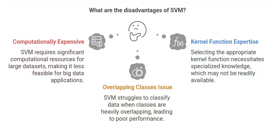
- SVM is computationally expensive for large datasets.
- Choosing the right kernel function requires expertise.
- It does not work well when classes are heavily overlapping.
4. How do I tune hyperparameters in SVM?
The two most important hyperparameters to tune are:
- C (Regularization parameter) - Controls trade-off between maximizing margin and minimizing misclassification.
- gamma (For RBF kernel) - Controls how far the influence of a training point reaches.
5. When should I use SVM instead of deep learning?
Use SVM when the dataset is small or medium-sized with well-defined features. Deep learning is better for large datasets with complex patterns.