What is Hierarchical Clustering? An Introduction to Hierarchical Clustering

1. Hierarchical Clustering
2. How Agglomerative Hierarchical clustering algorithm works
3. Euclidean Distance
4. Manhattan Distance
5. Minkowski Distance
6. Jaccard Similarity Coefficient/Jaccard Index
7. Cosine Similarity
8. Gower’s Similarity Coefficient 
9. Agglomerative clustering linkage algorithm (Cluster Distance Measure)
10. How to Find Optimal number of clustering

Contributed by: Satish Rajendran
LinkedIn Profile: https://www.linkedin.com/in/satish-rajendran85/

What is Hierarchical Clustering

Clustering is one of the popular techniques used to create homogeneous groups of entities or objects. For a given set of data points, grouping the data points into X number of clusters so that similar data points in the clusters are close to each other. 

In most of the analytical projects, after data cleaning and preparation, clustering techniques are often carried out before predictive or other analytical modeling.

Clustering falls under the category of unsupervised learning. Meaning, there is no labeled class or target variable for a given dataset. We are only interested in grouping similar records or objects in a cluster.

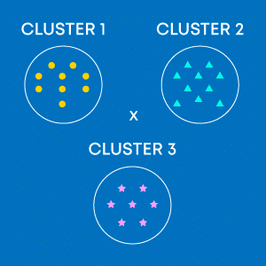
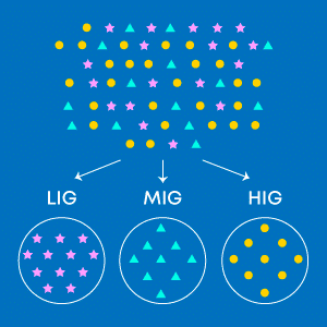
Let us try to understand clustering in r by taking a retail domain case study. Let’s say if the leading retail chain wanted to segregate customers into 3 categories, low-income group (LIG), medium-income group (MIG), and high-income group (HIG) based on their sales and customer data for better marketing strategies. 

In this case, data is available for all customers and the objective is to separate or form 3 different groups of customers. We can achieve this with the help of clustering techniques. The below image depicts the same. Pink, blue, and yellow circles are the data points which are grouped into 3 clusters, namely LIG, MIG, and HIG having similar type of customers or homogeneous group of customers within the clusters.

Now that we have a fair idea about clustering, it’s time to understand hierarchical clustering. 

Hierarchical Clustering creates clusters in a hierarchical tree-like structure (also called a Dendrogram). Meaning, a subset of similar data is created in a tree-like structure in which the root node corresponds to the entire data, and branches are created from the root node to form several clusters.

Also Read: Top 20 Datasets in Machine Learning

Hierarchical Clustering is of two types.

1. Divisive 
2. Agglomerative Hierarchical Clustering

Divisive Hierarchical Clustering is also termed as a top-down clustering approach. In this technique, entire data or observation is assigned to a single cluster. The cluster is further split until there is one cluster for each data or observation. 

Agglomerative Hierarchical Clustering is popularly known as a bottom-up approach, wherein each data or observation is treated as its cluster. A pair of clusters are combined until all clusters are merged into one big cluster that contains all the data.

Both algorithms are exactly the opposite of each other. So we will be covering Agglomerative Hierarchical clustering algorithms in detail. 

How Agglomerative Hierarchical clustering Algorithm Works

For a set of N observations to be clustered:

1. Start assigning each observation as a single point cluster, so that if we have N observations, we have N clusters, each containing just one observation. 
2. Find the closest (most similar) pair of clusters and make them into one cluster, we now have N-1 clusters. This can be done in various ways to identify similar and dissimilar measures (Explained in a later section)
3. Find the two closest clusters and make them to one cluster. We now have N-2 clusters. This can be done using agglomerative clustering linkage techniques (Explained in a later section)
4. Repeat steps 2 and 3 until all observations are clustered into one single cluster of size N.

Clustering algorithms use various distance or dissimilarity measures to develop different clusters. Lower/closer distance indicates that data or observation are similar and would get grouped in a single cluster. Remember that the higher the similarity depicts observation is similar.

Step 2 can be done in various ways to identify similar and dissimilar measures. Namely,

• Euclidean Distance
• Manhattan Distance
• Minkowski Distance
• Jaccard Similarity Coefficient
• Cosine Similarity
• Gower’s Similarity Coefficient 

Euclidean Distance

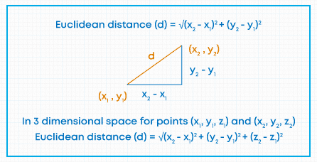
The Euclidean distance is the most widely used distance measure when the variables are continuous (either interval or ratio scale).

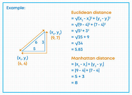
The Euclidean distance between two points calculates the length of a segment connecting the two points. It is the most evident way of representing the distance between two points.

The Pythagorean Theorem can be used to calculate the distance between two points, as shown in the figure below. If the points (x1, y1)) and (x2, y2) in 2-dimensional space, 

Then the Euclidean distance between them is as shown in the figure below.

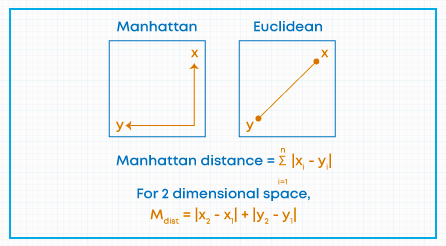
Manhattan Distance

Euclidean distance may not be suitable while measuring the distance between different locations. If we wanted to measure a distance between two retail stores in a city, then Manhattan distance will be more suitable to use, instead of Euclidean distance.

The distance between two points in a grid-based on a strictly horizontal and vertical path. The Manhattan distance is the simple sum of the horizontal and vertical components.

In nutshell, we can say Manhattan distance is the distance if you had to travel along coordinates only.

Minkowski Distance

The Minkowski distance between two variables X and Y is defined as-

When p = 1, Minkowski Distance is equivalent to the Manhattan distance, and the case where p = 2, is equivalent to the Euclidean distance.

Jaccard Similarity Coefficient/Jaccard Index

Jaccard Similarity Coefficient can be used when your data or variables are qualitative in nature. In particular to be used when the variables are represented in binary form such as (0, 1) or (Yes, No).

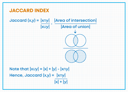
Where (X n Y) is the number of elements belongs to both X and Y

(X u Y) is the number of elements that belongs to either X or Y

We will try to understand with an example, note that we need to transform the data into binary form before applying Jaccard Index. Let’s consider Store 1 and Store 2 sell below items and each item is considered as an element.

Then, we can observe that bread, jam, coke and cake are sold by both stores. Hence, 1 is assigned for both stores.

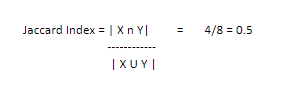
Jaccard Index value ranges from 0 to 1. Higher the similarity when Jaccard index is high.

Also Read: Overfitting and Underfitting in Machine Learning

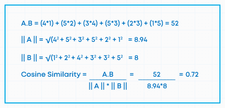
Cosine Similarity

Let A and B be two vectors for comparison. Using the cosine measure as a similarity function, we have-

Cosine Similarity values range between -1 and 1. Lower the cosine similarity, low is the similarity b/w two observations.

Let us understand by taking an example, consider shirt brand rating by 2 customer on the rate of 5 scale-

	Allen Solly	Arrow	Peter England	US Polo	Van Heusen	Zodiac
Customer 1	4	5	3	5	2	1
Customer 2	1	2	4	3	3	5

Gower’s Similarity Coefficient 

If the data contains both qualitative and quantitative variables then we cannot use any of the above distance and similarity measures as they are valid for qualitative or quantitative variables. Gower’s Similarity Coefficient can be used when data contains both qualitative and quantitative variables.

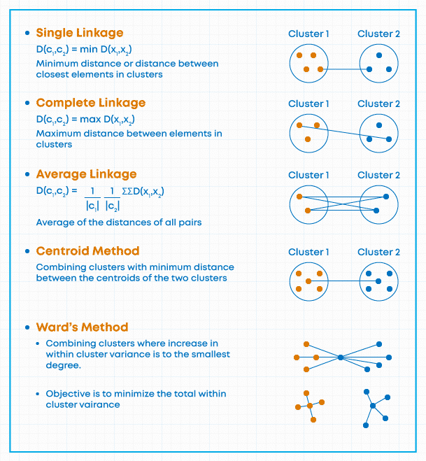
Agglomerative clustering linkage algorithm (Cluster Distance Measure)

This technique is used for combining two clusters. Note that it’s the distance between clusters, and not individual observation.

How to Find Optimal number of clustering

One of the challenging tasks in agglomerative clustering is to find the optimal number of clusters. Silhouette Score is one of the popular approaches for taking a call on the optimal number of clusters. It is a way to measure how close each point in a cluster is to the points in its neighboring clusters.

Let a_i be the mean distance between an observation i and other points in the cluster to which observation I assigned.

Let b_i be the minimum mean distance between an observation i and points in other clusters.

Silhouette Score ranges from -1 ro +1. Higher the value of Silhouette Score indicates observations are well clustered.

Silhouette Score = 1 indicates that the observation (i) is well matched in the cluster assignment.

This brings us to the end of the blog, if you found this helpful then enroll with Great Learning’s free Machine Learning foundation course!

You can also take up a free course on hierarchical clustering in r and upskill today!

While exploring machine hierarchical clustering, it’s essential to enhance your knowledge through comprehensive and structured online courses. Great Learning offers a range of free online certificate courses that can help you delve deeper into the fascinating world of data science and machine learning. These courses cover various topics such as clustering algorithms, data visualization, and more. By enrolling in these courses, you can gain valuable insights, practical skills, and hands-on experience, all at your own pace and convenience. Expand your understanding of machine hierarchical clustering and unlock new opportunities in the field of data science with Great Learning’s free online courses.