The LOOKUP function is one of Excel’s most helpful resources when you need to pull information from a list without scrolling through it manually. Whether you need to:
- Match IDs
- Find Prices
- Link Related Data
LOOKUP makes the process quick. In this tutorial, you’ll learn how to use the LOOKUP function step by step by understanding its syntax and using it in practical examples.
Learn Excel the smart way! Our course teaches you all the essential tools and techniques to master spreadsheets, from formulas to charts, and improve your workflow in every task you do.
What is the LOOKUP Function in Excel?
The LOOKUP function in Excel searches for a value in one range and returns a corresponding value from another range.
It helps you quickly find related information, such as matching a product ID to its price based on a lookup value.
Major Rule:
- LOOKUP requires your data to be sorted in ascending order (A-Z or Smallest to Largest).
- If your data is not sorted, the function may return incorrect results without showing an error.
How to Use the LOOKUP Function in Excel?
Excel might show you two options when you type the formula: Vector and Array.
- Vector Form (Recommended): Use this to search one row or column and find a result in a different row or column.
- Formula: =LOOKUP(lookup_value, lookup_vector, result_vector)
- Array Form: This is an older method provided for compatibility with other spreadsheet programs. It is rarely used today. It only works if the lookup data (array) has the lookup value in the first row or first column.
We will focus on the Vector form because it is much more flexible and easier to use.
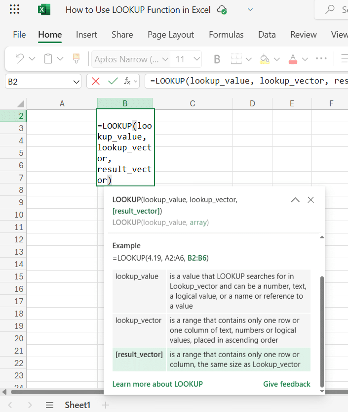
Explanation of Each Argument:
- lookup_value (required)
- This is the value you want to search for.
- It can be a number, text, or cell reference.
- Excel matches this value or returns the next smallest value in the sorted lookup_vector.
- lookup_vector (required)
- This is the one-dimensional range (either a row or column) where Excel will look for the lookup_value.
- Example: a list of marks, product prices, or age groups.
- result_vector (optional but typically used)
- This is the range from which Excel will return a result corresponding to the matched value in lookup_vector.
- It must be the same size and same orientation (row or column) as the lookup_vector.
If you omit the result_vector, Excel assumes that your lookup_vector is also your result source.
- How it behaves: Excel will search for the lookup_value in the lookup_vector and, once found, return that same value to you. This is useful if you simply want to confirm that a value exists in a list.
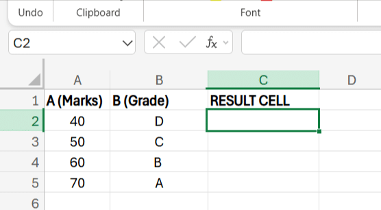
Step-by-Step Example
Suppose you are a teacher with a list of student marks and corresponding grades. You want to enter a student's score and have it automatically return their grade.
Data Table
Task:
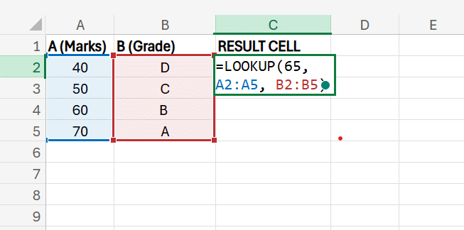
Look up a student’s score of 65 and find the appropriate grade.
Formula:
=LOOKUP(65, A2:A5, B2:B5)
Step-by-Step Explanation:
- Excel checks the lookup_vector → which is A2:A5 (marks).
- It tries to find an exact match for 65.
- Since 65 is not on the list, Excel looks for the largest value that is less than or equal to 65.
- In this case, it’s 60.
- Excel then identifies the position 60 in the lookup_vector, row 4 (A4).
- It returns the corresponding value from the same row in result_vector → B4, which is "B".
Final Output:
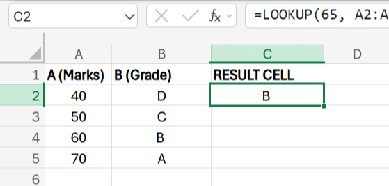
This tells us that a score of 65 earns a grade of "B".
Important Notes:
- If the lookup_value is less than the smallest value in the lookup_vector, the function returns #N/A.
- This function performs an approximate match, not an exact one, unless the value is exactly present.
New to Excel? Start with this free Excel for Beginners course to strengthen your Excel fundamentals.
Excel for Beginners Free Course
Learn essential Excel skills for data analysis, including functions, formulas, and data visualization techniques. Master cell referencing, sorting, and creating charts and presentations.
What Happens If the Value Isn’t Found?
There are two main cases where the LOOKUP function fails or gives incorrect results:
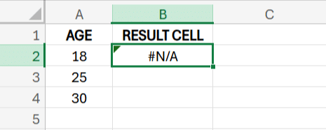
1. If lookup_value < all values in the lookup range:
Excel returns #N/A because there’s no value less than or equal to the lookup_value.
Example:
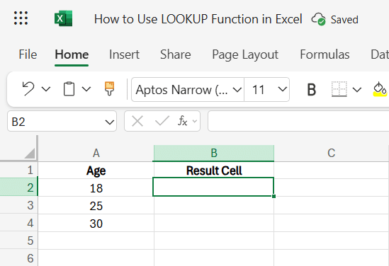
Formula
=LOOKUP(16, A2:A4)
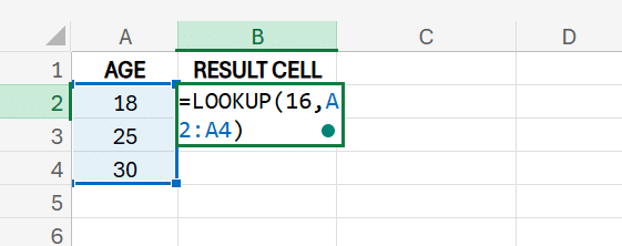
- Since 16 is smaller than the lowest value (18), the result will be: #N/A
2. If the lookup vector is not sorted:
- The function will not show an error, but may return the wrong result.
Summary Table: How LOOKUP Handles Value Matching
| Scenario | Result | Notes |
| Exact match found | Returns match | Standard behavior |
| No exact match, a smaller value exists | Returns the nearest smaller match | Only if the data is sorted in ascending order |
| No smaller value exists | #N/A | Lookup value is less than all entries |
| Data not sorted | Unreliable result | May return the wrong value or unexpected output |
Learn Excel the smart way! Our course teaches you all the essential tools and techniques to master spreadsheets, from formulas to charts, and improve your workflow in every task you do.
Tips and Best Practices for Using the LOOKUP Function in Excel
1. Use LOOKUP Only When Approximate Matching Is Acceptable
- LOOKUP is designed for approximate matches by default.
- Use VLOOKUP, HLOOKUP, or XLOOKUP if you need exact matches.
2. Use Descriptive Named Ranges for Better Readability
- Define named ranges and result vectors for your lookup.
- This makes formulas easier to understand and manage.
Example:
=LOOKUP(ProductID, ProductIDs, Prices)
3. Avoid Using LOOKUP with Volatile or Frequently Changing Data
- LOOKUP relies on sorted data and approximate matching; it may not adapt well to datasets that change often or include dynamic user inputs.
4. Document Your Formula Logic
- Add comments or cell notes explaining what your LOOKUP formula does.
- This is especially helpful in shared or complex spreadsheets.
Learning the LOOKUP function in Excel can be a useful tool for effective data analysis, as it helps you quickly find data as per your query.
For those who want to strengthen their skills in using various Excel formulas for assigned tasks, Great Learning’s Data Analytics in Excel course provides hands-on training to help you become better at handling data and extracting meaningful insights from complex datasets that support data-driven decision-making for organizational growth.
Learn Excel for powerful data analysis and enhance your skills for better decision-making.