Multinomial Naive Bayes Explained

1. Introduction to Multinomial Naïve Bayes
2. The Bag of Words Model
3. Difference between Bernoulli, Multinomial and Gaussian Naïve Bayes
4. Advantages
5. Disadvantages
6. Applications

Contributed by: Gautam Solanki
LinkedIn Profile: https://www.linkedin.com/in/gautam-solanki-05b988a2/

Introduction

With an ever-growing amount of textual information stored in electronic form such as legal documents, policies, company strategies, etc., automatic text classification is becoming increasingly important. This requires a supervised learning technique that classifies every new document by assigning one or more class labels from a fixed or predefined class. It uses the bag of words approach, where the individual words in the document constitute its features, and the order of the words is ignored. This technique is different from the way we communicate with each other. It treats the language like it’s just a bag full of words and each message is a random handful of them. Large documents have a lot of words that are generally characterized by very high dimensionality feature space with thousands of features. Hence, the learning algorithm requires to tackle high dimensional problems, both in terms of classification performance and computational speed. 

Naïve Bayes, which is computationally very efficient and easy to implement, is a learning algorithm frequently used in text classification problems. Two event models are commonly used: 

• Multivariate Bernoulli Event Model
• Multivariate Event Model

The Multivariate Event model is referred to as Multinomial Naive Bayes.

When most people want to learn about Naive Bayes, they want to learn about the Multinomial Naive Bayes Classifier. However, there is another commonly used version of Naïve Bayes, called Gaussian Naive Bayes Classification. Check out the free course on naive Bayes supervised learning.

Naive Bayes is based on Bayes’ theorem, where the adjective Naïve says that features in the dataset are mutually independent. Occurrence of one feature does not affect the probability of occurrence of the other feature. For small sample sizes, Naïve Bayes can outperform the most powerful alternatives. Being relatively robust, easy to implement, fast, and accurate, it is used in many different fields. Check out naïve bayes classifiers.

For Example, Spam filtering in email, Diagnosis of diseases, making decisions about treatment, Classification of RNA sequences in taxonomic studies, to name a few. However, we have to keep in mind about the type of data and the type of problem to be solved that dictates which classification model we want to choose. Strong violations of the independence assumptions and non-classification problems can lead to poor performance. In practice, it is recommended to use different classification models on the same dataset and then consider the performance, as well as computational efficiency.

Also Read: Top Machine Learning Interview Questions

To understand how Naïve Bayes works, first, we have to understand the concept of Bayes’ rule. This probability model was formulated by Thomas Bayes (1701-1761) and can be written as:

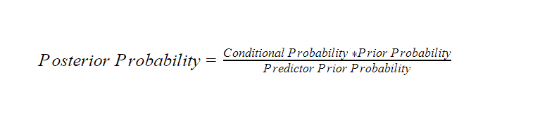
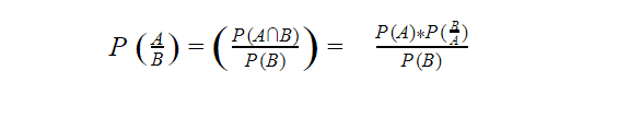
where,
PA= the prior probability of occurring A
PBA= the condition probability of B given that A occurs
PAB= the condition probability of A given that B occurs
PB= the probability of occuring B

The posterior probability, can be interpreted as: What is the revised probability of an event occurring after taking new information into consideration?

It is a better reflection of the underlying truth of a data generating process because it includes more information.

Conditional Probability

The probability of one event A occurring when another event B with some relationship to A has already occurred is called conditional probability.

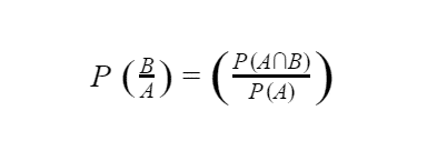
This expression is valid only when P(A) is greater than zero.

Prior Probability

This probability can be defined as the prior knowledge or belief i.e. the probability of an event computed before the collection of new data. This probability is revised as new information becomes available to produce more accurate results.

If the prior observations are used to calculate the probability, we call it prior probability.

The Bag of Words Model

Feature extraction and Selection are the most important sub-tasks in pattern classification. The three main criteria of good features are:

1. Salient: The features should be meaningful and important to the problem
2. Invariant: The features are resistant to scaling, distortion and orientation etc. 
3. Discriminatory:  For training of classifiers, the features should have enough information to distinguish between patterns.

Bag of words is a commonly used model in Natural Language Processing. The idea behind this model is the creation of vocabulary that contains the collection of different words, and each word is associated with a count of how it occurs. Later, the vocabulary is used to create d-dimensional feature vectors.

For Example: 

D1: Each country has its own constitution
D2: Every country has its own uniqueness

Vocabulary could be written as:
V= {each : 1, state : 1, has : 2, its : 2, own : 2, constitution : 1, every : 1, country : 2,} 

Tokenization

It is the process of breaking down the text corpus into individual elements. These individual elements act as an input to machine learning algorithms.

For Example:

Every country has its own uniqueness 

Stop Words

Stop Words also known as un-informative words such as (so, and, or, the) should be removed from the document.

Stemming and Lemmatization

Stemming and Lemmatization are the process of transforming a word into its root form and aims to obtain the grammatically correct forms of words.

The above-mentioned process comes under the Bag of Words Model. Multinomial Naïve Bayes uses term frequency i.e. the number of times a given term appears in a document. Term frequency is often normalized by dividing the raw term frequency by the document length. After normalization, term frequency can be used to compute maximum likelihood estimates based on the training data to estimate the conditional probability.

Example:

Let me explain a Multinomial Naïve Bayes Classifier where we want to filter out the spam messages. Initially, we consider eight normal messages and four spam messages. Now, imagine we received a lot of emails from friends, family, office and we also received spam (unwanted messages that are usually scams or unsolicited advertisements). 

Let see the histogram of all the words that occur in the normal messages from family and friends.

We can use the histogram to calculate the probabilities of seeing each word, given that it was a normal message. The probability of word dear given that we saw in normal message is-

Probability (Dear|Normal) = 8 /17 = 0.47

Similarly, the probability of word Friend is-

Probability (Friend/Normal) = 5/ 17 =0.29
Probability (Lunch/Normal) = 3/ 17 =0.18
Probability (Money/Normal) = 1/ 17 =0.06

Now let’s make the histogram of all the words in spam.

The probability of word dear given that we saw in spam message is-

Probability (Dear|Spam) = 2 /7 = 0.29

Similarly, the probability of word Friend is-

Probability (Friend/Spam) = 1/ 7 =0.14
Probability (Lunch/Spam) = 0/ 7 =0.00
Probability (Money/Spam) = 4/ 7 =0.57

Here, we have calculated the probabilities of discrete words and not the probability of something continuous like weight or height. These Probabilities are also called Likelihoods.

Now, let’s say we have received a normal message as Dear Friend and we want to find out if it’s a normal message or spam. 

We start with an initial guess that any message is a Normal Message.

From our initial assumptions of 8 Normal messages and 4 Spam messages, 8 out of 12 messages are normal messages. The prior probability, in this case, will be:

Probability (Normal) = 8 / (8+4) = 0.67

We multiply this prior probability with the probabilities of Dear Friend that we have calculated earlier.

0.67 * 0.47 * 0.29 = 0.09

0.09 is the probability score considering Dear Friend is a normal message. 

Alternatively, let’s say that any message is a Spam.

4 out of 12 messages are Spam. The prior probability in this case will be:

Probability (Normal) = 4 / (8+4) = 0.33

Now we multiply the prior probability with the probabilities of Dear Friend that we have calculated earlier.

0.33 * 0.29 * 0.14 = 0.01

0.01 is the probability score considering Dear Friend is a Spam. 

The probability score of Dear Friend being a normal message is greater than the probability score of Dear Friend being spam. We can conclude that Dear Friend is a normal message.

Naive Bayes treats all words equally regardless of how they are placed because it’s difficult to keep track of every single reasonable phrase in a language.

Difference between Bernoulli, Multinomial and Gaussian Naive Bayes

Multinomial Naïve Bayes consider a feature vector where a given term represents the number of times it appears or very often i.e. frequency. On the other hand, Bernoulli is a binary algorithm used when the feature is present or not. At last Gaussian is based on continuous distribution.

Advantages:

1. Low computation cost.
2. It can effectively work with large datasets.
3. For small sample sizes, Naive Bayes can outperform the most powerful alternatives.
4. Easy to implement, fast and accurate method of prediction.
5. Can work with multiclass prediction problems.
6. It performs well in text classification problems.

Disadvantages:

It is very difficult to get the set of independent predictors for developing a model using Naive Bayes.

Applications:

1. Naive Bayes classifier is used in Text Classification, Spam filtering and Sentiment Analysis. It has a higher success rate than other algorithms.
2. Naïve Bayes along with Collaborative filtering are used in Recommended Systems.
3. It is also used in disease prediction based on health parameters.
4. This algorithm has also found its application in Face recognition.
5. Naive Bayes is used in prediction of weather reports based on atmospheric conditions (temp, wind, clouds, humidity etc.)

This brings us to the end of the blog about Multinomial Naïve Bayes. To learn more such concepts, you can upskill with Great Learning Academy’s free online courses.