R Tutorial

Introduction to R

R is a programming language developed by Ross Ihaka and Robert Gentleman in 1993. R possesses an extensive catalog of statistical and graphical methods. It includes machine learning algorithms, linear regression, time series, and statistical inference, to name a few. Most R libraries are written in R, but C, C++, and Fortran codes are preferred for heavy computational tasks.

Data analysis with R is done in a series of steps; programming, transforming, discovering, modeling, and communicating the results

• Program: R is a clear and accessible programming tool
• Transform: R is made up of a collection of libraries designed specifically for data science
• Discover: Investigate the data, refine your hypothesis and analyze them
• Model: R provides a wide array of tools to capture the right model for your data
• Communicate: Integrate codes, graphs, and outputs to a report with R Markdown or build Shiny apps to share with the world.

Check out the free R in Data Science course to learn more about the significant concepts of R from scratch.

What is R used for?

• Statistical inference
• Data analysis
• Machine learning algorithm

As conclusion, R is the world’s most widely used statistics programming language. It’s the 1st choice of data scientists and supported by a vibrant and talented community of contributors. R is taught in universities and deployed in mission-critical business applications.

R-environment setup

Windows Installation – We can download the Windows installer version of R from R-3.2.2 for windows (32/64)

As it is a Windows installer (.exe) with the name “R-version-win.exe”. You can just double click and run the installer accepting the default settings. If your Windows is a 32-bit version, it installs the 32-bit version. But if your windows are 64-bit, then it installs both the 32-bit and 64-bit versions.

After installation, you can locate the icon to run the program in a directory structure “RR3.2.2bini386Rgui.exe” under the Windows Program Files. Clicking this icon brings up the R-GUI which is the R console to do R Programming. 

R basic Syntax

R Programming is a popular programming language broadly used in data analysis. The way in which we define its code is quite simple. The “Hello World!” is the basic program for all the languages, and now we will understand the syntax of R programming with the “Hello world” program. We can write our code either in the command prompt, or we can use an R script file.

R command prompt

Once you have R environment setup, then it’s easy to start your R command prompt by just typing the following command at your command prompt −
$R
This will launch R interpreter and you will get a prompt > where you can start typing your program as follows −

>myString <- "Hello, World"
>print (myString)
[1] "Hello, World!"

Here the first statement defines a string variable myString, where we assign a string “Hello, World!” and then the next statement print() is being used to print the value stored in myString variable.

R data-types

While doing programming in any programming language, you need to use various variables to store various information. Variables are nothing but reserved memory locations to store values. This means that when you create a variable you reserve some space in memory.

In contrast to other programming languages like C and java in R, the variables are not declared as some data type. The variables are assigned with R-Objects and the data type of the R-object becomes the variable’s data type. There are many types of R-objects. The frequently used ones are −

• Vectors
• Lists
• Matrices
• Arrays
• Factors
• Data Frames

Vectors

#create a vector and find the elements which are >5
v<-c(1,2,3,4,5,6,5,8)
v[v>5]

#subset
subset(v,v>5)

#position in the vector created in which square of the numbers of v is >10 holds good
which(v*v>10)

#to know the values 
v[v*v>10]

Output: [1] 6 8

Output: [1] 6 8

Output: [1] 4 5 6 7 8

Output: [1] 4 5 6 5 8

Matrices

A matrix is a two-dimensional rectangular data set. It can be created using a vector input to the matrix function.

#matrices: a vector with two dimensional attributes
mat<-matrix(c(1,2,3,4))
 
mat1<-matrix(c(1,2,3,4),nrow=2)
mat1

Output:     [,1] [,2]
 [1,]    1    3
 [2,]    2    4

mat2<-matrix(c(1,2,3,4),ncol=2,byrow=T)
mat2

Output:       [,1] [,2]
 [1,]    1    2
 [2,]    3    4

mat3<-matrix(c(1,2,3,4),byrow=T)
mat3

#transpose of matrix
mattrans<-t(mat)
mattrans

#create a character matrix called fruits with elements apple, orange, pear, grapes
fruits<-matrix(c("apple","orange","pear","grapes"),2)
#create 3×4 matrix of marks obtained in each quarterly exams for 4 different subjects 
X<-matrix(c(50,70,40,90,60, 80,50, 90,100, 50,30, 70),nrow=3)
X

#give row names and column names
rownames(X)<-paste(prefix="Test.",1:3)
subs<-c("Maths", "English", "Science", "History")
colnames(X)<-subs
X

Output:       [,1]  [1,]    1  [2,]    2  [3,]    3  [4,]    4 Output:      [,1] [,2] [,3] [,4]  [1,]    1    2    3    4 Output:      [,1] [,2] [,3] [,4]  [1,]   50   90   50   50  [2,]   70   60   90   30  [3,]   40   80  100   70 Output:   Maths English Science History  Test. 1    50      90      50      50  Test. 2    70      60      90      30  Test. 3    40      80     100      70

Arrays

While matrices are confined to two dimensions, arrays can be of any number of dimensions. The array function takes a dim attribute, creating the required dimensions. In the below example, we create an array with two elements which are 3×3 matrices each.

#Arrays
arr<-array(1:24,dim=c(3,4,2))
arr

#create an array using alphabets with dimensions 3 rows, 2 columns and 3 arrays
arr1<-array(letters[1:18],dim=c(3,2,3))

#select only 1st two matrix of an array
arr1[,,c(1:2)]

#LIST
X<-list(u=2, n='abc')
X
X$u

Output: , , 1
  [,1] [,2] [,3] [,4]
 [1,]    1    4    7   10
 [2,]    2    5    8   11
 [3,]    3    6    9   12
 , , 2
  [,1] [,2] [,3] [,4]
 [1,]   13   16   19   22
 [2,]   14   17   20   23
 [3,]   15   18   21   24

Output: 
 , , 1
  [,1] [,2]
 [1,] "a"  "d" 
 [2,] "b"  "e" 
 [3,] "c"  "f" 
 , , 2
  [,1] [,2]
 [1,] "g"  "j" 
 [2,] "h"  "k" 
 [3,] "i"  "l" 
 arr1[,,3]
 Output:       [,1] [,2]
 [1,] "m"  "p" 
 [2,] "n"  "q" 
 [3,] "o"  "r" 

Output:
  $u
 [1] 2
 $n
 [1] "abc"

Dataframes

Data frames are tabular data objects. Unlike a matrix in a data frame, each column can contain different modes of data. The first column can be numeric while the second column can be character and the third column can be logical. It is a list of vectors of equal length.

#Dataframes
students<-c("J","L","M","K","I","F","R","S")
Subjects<-rep(c("science","maths"),each=2)
marks<-c(55,70,66,85,88,90,56,78)
data<-data.frame(students,Subjects,marks)
#Accessing dataframes
data[[1]]

data$Subjects
data[,1]

Output: 
 [1] J L M K I F R S
 Levels: F I J K L M R S

Output: 
   data$Subjects
   [1] science science maths   maths   science science maths   maths  
   Levels: maths science 

Factors

Factors are the r-objects that are created using a vector. It stores the vector along with the distinct values of the elements in the vector as labels. The labels are always characters irrespective of whether it is numeric or character or Boolean etc. in the input vector. They are useful in statistical modeling.

Factors are created using the factor() function. The nlevels function gives the count of levels.

#Factors
x<-c(1,2,3)
factor(x)

#apply function
data1<-data.frame(age=c(55,34,42,66,77),bmi=c(26,25,21,30,22))
d<-apply(data1,2,mean)
d

#create two vectors age and gender and find mean age with respect to gender
age<-c(33,34,55,54)
gender<-factor(c("m","f","m","f"))
tapply(age,gender,mean)

Output: [1] 1 2 3
 Levels: 1 2 3

Output:  age  bmi 
 54.8 24.8 

Output:  f  m 
         44 44

R Variables

A variable provides us with named storage that our programs can manipulate. A variable in R can store an atomic vector, a group of atomic vectors, or a combination of many R objects. A valid variable name consists of letters, numbers, and the dot or underlined characters.

Rules for writing Identifiers in R

1. Identifiers can be a combination of letters, digits, period (.), and underscore (_).
2. It must start with a letter or a period. If it starts with a period, it cannot be followed by a digit.
3. Reserved words in R cannot be used as identifiers.

Valid identifiers in R

total, sum, .fine.with.dot, this_is_acceptable, Number5

Invalid identifiers in R

tot@l, 5um, _fine, TRUE, .0ne

Best Practices

Earlier versions of R used underscore (_) as an assignment operator. So, the period (.) was used extensively in variable names having multiple words. Current versions of R support underscore as a valid identifier, but it is good practice to use a period as word separator.
For example, a.variable.name is preferred over a_variable_name or alternatively, we could use camel case as aVariableName.

Constants in R

As the name suggests, constants are entities whose value cannot be altered. The basic types of constants are numeric constants and character constants.

Numeric Constants

All numbers fall under this category. They can be of type integer, double or complex. It can be checked with the typeof() function.
Numeric Constants followed by L are regarded as integers and those followed by i are regarded as complex.

> typeof(5)
> typeof(5L)
> typeof(5L)

[1] “double”
[1] “double”
[[1] “double”

Character Constants

Character constants can be represented using either single quotes (‘) or double quotes (“) as delimiters.

> 'example'
> typeof("5")

[1] "example"
[1] "character"

R Operators

Operators – Arithmetic, Relational, Logical, Assignment, and some of the Miscellaneous Operators that R programming language provides. 

There are four main categories of Operators in the R programming language.

1. Arithmetic Operators
2. Relational Operators
3. Logical Operators
4. Assignment Operators
5. Mixed Operators

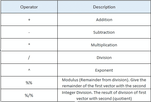
x <- 35
y<-10

   x+y       > x-y     > x*y       > x/y      > x%/%y     > x%%y   > x^y
   [1] 45      [1] 25    [1] 350    [1] 3.5      [1] 3      [1] 5 [1]2.75e+15 

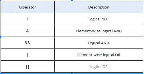
Logical Operators

The below table shows the logical operators in R. Operators & and | perform element-wise operation producing result having a length of the longer operand. But && and || examines only the first element of the operands resulting in a single length logical vector.

a <- c(TRUE,TRUE,FALSE,0,6,7)
b <- c(FALSE,TRUE,FALSE,TRUE,TRUE,TRUE)
a&b 
[1] FALSE TRUE FALSE FALSE TRUE TRUE
a&&b
[1] FALSE
> a|b
[1] TRUE TRUE FALSE TRUE TRUE TRUE
> a||b
[1] TRUE
> !a
[1] FALSE FALSE TRUE TRUE FALSE FALSE
> !b
[1] TRUE FALSE TRUE FALSE FALSE FALSE

R functions

Functions are defined using the function() directive and stored as R objects like anything else. In particular, they are R objects of class “function”. Here’s a simple function that takes no arguments and simply prints ‘Hi statistics’.

#define the function
f <- function() {
print("Hi statistics!!!")
}
#Call the function
f()

Output:
 [1] "Hi statistics!!!"

Now let’s define a function called standardize, and the function has a single argument x which is used in the body of a function.

#Define the function that will calculate standardized score.
standardize = function(x) {
m = mean(x)
sd = sd(x)
result = (x – m) / sd
result
}
input<- c(40:50) #Take input for what we want to calculate a standardized score.
standardize(input) #Call the function

Output: 
   standardize(input) #Call the function
   [1] -1.5075567 -1.2060454 -0.9045340 -0.6030227 -0.3015113 0.0000000 0.3015113 0.6030227 0.9045340 1.2060454 1.5075567 

Loop Functions

R has some very useful functions which implement looping in a compact form to make life easier. The very rich and powerful family of applied functions is made of intrinsically vectorized functions. These functions in R allow you to apply some function to a series of objects (eg. vectors, matrices, data frames, or files). They include:

1. lapply(): Loop over a list and evaluate a function on each element
2. sapply(): Same as lapply() but try to simplify the result
3. apply(): Apply a function over the margins of an array
4. tapply(): Apply a function over subsets of a vector
5. mapply(): Multivariate version of lapply

There is another function called split(), which is also useful, particularly in conjunction with lapply.

R Vectors

A vector is a sequence of data elements of the same basic type. Members in a vector are officially called components. Vectors are the most basic R data objects, and there are six types of atomic vectors. They are logical, integer, double, complex, character, and raw.

The c() function can be used to create vectors of objects by concatenating things together. 
x <- c(1,2,3,4,5) #double
x #If you use only x auto-printing occurs
l <- c(TRUE, FALSE) #logical
l <- c(T, F) ## logical
c <- c("a", "b", "c", "d") ## character
i <- 1:20 ## integer
cm <- c(2+2i, 3+3i) ## complex
print(l)
print(c)
print(i)
print(cm)

You can see the type of each vector using typeof() function in R.
typeof(x)
typeof(l)
typeof(c)
typeof(i)
typeof(cm)

Output:
 print(l)
 [1] TRUE FALSE
   print(c)
   [1] "a" "b" "c" "d"
   print(i)
   [1] 1 2 3 4 5 6 7 8 9 10 11 12 13 14 15 16 17 18 19 20
   print(cm)
   [1] 2+2i 3+3i 

Output: 
 typeof(x)
 [1] "double"
   typeof(l)
   [1] "logical"
   typeof(c)
   [1] "character"
   typeof(i)
   [1] "integer"
   typeof(cm)
   [1] "complex" 

Creating a vector using seq() function:

We can use the seq() function to create a vector within an interval by specifying step size or specifying the length of the vector. 

seq(1:10) #By default it will be incremented by 1
seq(1, 20, length.out=5) # specify length of the vector
seq(1, 20, by=2) # specify step size

Output:
 > seq(1:10) #By default it will be incremented by 1
 [1] 1 2 3 4 5 6 7 8 9 10
 > seq(1, 20, length.out=5) # specify length of the vector
 [1] 1.00 5.75 10.50 15.25 20.00
 > seq(1, 20, by=2) # specify step size
 [1] 1 3 5 7 9 11 13 15 17 19

Extract Elements from a Vector:

Elements of a vector can be accessed using indexing. The vector indexing can be logical, integer, or character. The [ ] brackets are used for indexing. Indexing starts with position 1, unlike most programming languages, where indexing starts from 0.

Extract Using Integer as Index:

We can use integers as an index to access specific elements. We can also use negative integers to return all elements except that specific element.

x<- 101:110
x[1]   #access the first element
x[c(2,3,4,5)] #Extract 2nd, 3rd, 4th, and 5th elements
x[5:10]        #Extract all elements from 5th to 10th
x[c(-5,-10)] #Extract all elements except 5th and 10th
x[-c(5:10)] #Extract all elements except from 5th to 10th 

Output:
   x[1] #Extract the first element
   [1] 101
   x[c(2,3,4,5)] #Extract 2nd, 3rd, 4th, and 5th elements
   [1] 102 103 104 105
   x[5:10] #Extract all elements from 5th to 10th
   [1] 105 106 107 108 109 110
   x[c(-5,-10)] #Extract all elements except 5th and 10th
   [1] 101 102 103 104 106 107 108 109
   x[-c(5:10)] #Extract all elements except from 5th to 10th
   [1] 101 102 103 104 

Extract Using Logical Vector as Index:

If you use a logical vector for indexing, the position where the logical vector is TRUE will be returned.

x[x < 105]
x[x>=104]

Output: 
   x[x < 105] [1] 101 102 103 104 
x[x>=104]
   [1] 104 105 106 107 108 109 110 

Modify a Vector in R:

We can modify a vector and assign a new value to it. You can truncate a vector by using reassignments. Check the below example. 

x<- 10:12
x[1]<- 101 #Modify the first element
x
x[2]<-102 #Modify the 2nd element
x
x<- x[1:2] #Truncate the last element
x 

Output: 
   x
   [1] 101 11 12
   x[2]<-102 #Modify the 2nd element
   x
   [1] 101 102 12
   x<- x[1:2] #Truncate the last element
   x
   [1] 101 102 

Arithmetic Operations on Vectors:

We can use arithmetic operations on two vectors of the same length. They can be added, subtracted, multiplied, or divided. Check the output of the below code.

# Create two vectors.
v1 <- c(1:10)
v2 <- c(101:110)

# Vector addition.
add.result <- v1+v2
print(add.result)
# Vector subtraction.
sub.result <- v2-v1
print(sub.result)
# Vector multiplication.
multi.result <- v1*v2
print(multi.result)
# Vector division.
divi.result <- v2/v1
print(divi.result)

Output:
   print(add.result)
   [1] 102 104 106 108 110 112 114 116 118 120
   print(sub.result)
   [1] 100 100 100 100 100 100 100 100 100 100
   print(multi.result)
   [1] 101 204 309 416 525 636 749 864 981 1100
   print(divi.result)
   [1] 101.00000 51.00000 34.33333 26.00000 21.00000 17.66667 15.28571 13.50000 12.11111 11.00000 

Find Minimum and Maximum in a Vector:

A vector’s minimum and maximum can be found using the min() or the max() function. range() is also available, which returns the minimum and maximum in a vector.

x<- 1001:1010
max(x) # Find the maximum
min(x) # Find the minimum
range(x) #Find the range

Output: 
   max(x) # Find the maximum
   [1] 1010
   min(x) # Find the minimum
   [1] 1001
   range(x) #Find the range
   [1] 1001 1010 

R Lists

The list is a data structure having elements of mixed data types. A vector having all elements of the same type is called an atomic vector but a vector having elements of a different type is called list.
We can check the type with typeof() or class() function and find the length using length()function.

x <- list("stat",5.1, TRUE, 1 + 4i)
x
class(x)
typeof(x)
length(x)

Output:
   x
   [[1]]
   [1] "stat"
   [[2]]
   [1] 5.1
   [[3]]
   [1] TRUE
   [[4]]
   [1] 1+4i
   class(x)
   [1] “list”
   typeof(x)
   [1] “list”
   length(x)
   [1] 4 

You can create an empty list of a prespecified length with the vector() function.

x <- vector("list", length = 10)
x

Output:
   x
   [[1]]
   NULL
   [[2]]
   NULL
   [[3]]
   NULL
   [[4]]
   NULL
   [[5]]
   NULL
   [[6]]
   NULL
   [[7]]
   NULL
   [[8]]
   NULL
   [[9]]
   NULL
   [[10]]
   NULL 

How to extract elements from a list?

Lists can be subsets using two syntaxes, the $ operator and square brackets []. The $ operator returns a named element of a list. The [] syntax returns a list, while the [[]] returns an element of a list.

# subsetting
l$e
l["e"]
l[1:2]
l[c(1:2)] #index using integer vector
l[-c(3:length(l))] #negative index to exclude elements from 3rd up to last.
l[c(T,F,F,F,F)] # logical index to access elements

Output:
 > l$e
 [,1] [,2] [,3] [,4] [,5] [,6] [,7] [,8] [,9] [,10]
 [1,] 1 0 0 0 0 0 0 0 0 0
 [2,] 0 1 0 0 0 0 0 0 0 0
 [3,] 0 0 1 0 0 0 0 0 0 0
 [4,] 0 0 0 1 0 0 0 0 0 0
 [5,] 0 0 0 0 1 0 0 0 0 0
 [6,] 0 0 0 0 0 1 0 0 0 0
 [7,] 0 0 0 0 0 0 1 0 0 0
 [8,] 0 0 0 0 0 0 0 1 0 0
 [9,] 0 0 0 0 0 0 0 0 1 0
 [10,] 0 0 0 0 0 0 0 0 0 1
 > l["e"]
 $e
 [,1] [,2] [,3] [,4] [,5] [,6] [,7] [,8] [,9] [,10]
 [1,] 1 0 0 0 0 0 0 0 0 0
 [2,] 0 1 0 0 0 0 0 0 0 0
 [3,] 0 0 1 0 0 0 0 0 0 0
 [4,] 0 0 0 1 0 0 0 0 0 0
 [5,] 0 0 0 0 1 0 0 0 0 0
 [6,] 0 0 0 0 0 1 0 0 0 0
 [7,] 0 0 0 0 0 0 1 0 0 0
 [8,] 0 0 0 0 0 0 0 1 0 0
 [9,] 0 0 0 0 0 0 0 0 1 0
 [10,] 0 0 0 0 0 0 0 0 0 1
 > l[1:2]
 [[1]]
 [1] 1 2 3 4
 [[2]]
 [1] FALSE
 > l[c(1:2)] #index using integer vector
 [[1]]
 [1] 1 2 3 4
 [[2]]
 [1] FALSE
 > l[-c(3:length(l))] #negative index to exclude elements from 3rd up to last.
 [[1]]
 [1] 1 2 3 4
 [[2]]
 [1] FALSE
 l[c(T,F,F,F,F)]
 [[1]]
 [1] 1 2 3 4

Modifying a List in R:

We can change components of a list through reassignment.

l[["name"]] <- "Kalyan Nandi"
l

Output:
 [[1]]
 [1] 1 2 3 4
 [[2]]
 [1] FALSE
 [[3]]
 [1] “Hello Statistics!”
 $d
 function (arg = 42)
 {
 print(“Hello World!”)
 }
 $name
 [1] “Kalyan Nandi”

R Matrices

In R Programming Matrix is a two-dimensional data structure. They contain elements of the same atomic types. A Matrix can be created using the matrix() function. R can also be used for matrix calculations. Matrices have rows and columns containing a single data type. In a matrix, the order of rows and columns is important. Dimension can be checked directly with the dim() function, and all attributes of an object can be checked with the attributes() function. Check the below example.

Creating a matrix in R

m <- matrix(nrow = 2, ncol = 3)
dim(m)
attributes(m)
m <- matrix(1:20, nrow = 4, ncol = 5)
m

Output:
   dim(m)
   [1] 2 3
   attributes(m)
   $dim
   [1] 2 3
   m <- matrix(1:20, nrow = 4, ncol = 5)
   m
   [,1] [,2] [,3] [,4] [,5]
   [1,] 1 5 9 13 17
   [2,] 2 6 10 14 18
   [3,] 3 7 11 15 19
   [4,] 4 8 12 16 20 

Matrices can be created by column-binding or row-binding with the cbind() and rbind() functions.

x<-1:3
y<-10:12
z<-30:32
cbind(x,y,z)
rbind(x,y,z)

Output:
   cbind(x,y,z)
   x y z
   [1,] 1 10 30
   [2,] 2 11 31
   [3,] 3 12 32
   rbind(x,y,z)
   [,1] [,2] [,3]
   x 1 2 3
   y 10 11 12
   z 30 31 32 

By default, the matrix function reorders a vector into columns, but we can also tell R to use rows instead.

x <-1:9
matrix(x, nrow = 3, ncol = 3)
matrix(x, nrow = 3, ncol = 3, byrow = TRUE)

Output
   cbind(x,y,z)
   x y z
   [1,] 1 10 30
   [2,] 2 11 31
   [3,] 3 12 32
   rbind(x,y,z)
   [,1] [,2] [,3]
   x 1 2 3
   y 10 11 12
   z 30 31 32 

R Arrays

In R, Arrays are the data types that can store data in more than two dimensions. An array can be created using the array() function. It takes vectors as input and uses the values in the dim parameter to create an array. If you create an array of dimensions (2, 3, 4) then it creates 4 rectangular matrices each with 2 rows and 3 columns. Arrays can store only data types.

Give a Name to Columns and Rows:

We can give names to the array’s rows, columns, and matrices by setting the dimnames parameter.

v1 <- c(1,2,3)
v2 <- 100:110
col.names <- c("Col1","Col2","Col3","Col4","Col5","Col6","Col7")
row.names <- c("Row1","Row2")
matrix.names <- c("Matrix1","Matrix2")
arr4 <- array(c(v1,v2), dim=c(2,7,2), dimnames = list(row.names,col.names, matrix.names))
arr4

Output:
 , , Matrix1
 Col1 Col2 Col3 Col4 Col5 Col6 Col7
 Row1 1 3 101 103 105 107 109
 Row2 2 100 102 104 106 108 110
 , , Matrix2
 Col1 Col2 Col3 Col4 Col5 Col6 Col7
 Row1 1 3 101 103 105 107 109
 Row2 2 100 102 104 106 108 110

Accessing/Extracting Array Elements:

# Print the 2nd row of the 1st matrix of the array.
print(arr4[2,,1])
# Print the element in the 2nd row and 4th column of the 2nd matrix.
print(arr4[2,4,2])
# Print the 2nd Matrix.
print(arr4[,,2])

Output:
 > print(arr4[2,,1])
 Col1 Col2 Col3 Col4 Col5 Col6 Col7
 2 100 102 104 106 108 110
 >
 > # Print the element in the 2nd row and 4th column of the 2nd matrix.
 > print(arr4[2,4,2])
 [1] 104
 >
 > # Print the 2nd Matrix.
 > print(arr4[,,2])
 Col1 Col2 Col3 Col4 Col5 Col6 Col7
 Row1 1 3 101 103 105 107 109
 Row2 2 100 102 104 106 108 110

R Factors

Factors are used to represent categorical data and can be unordered or ordered. An example might be “Male” and “Female” if we consider gender. Factor objects can be created with the factor() function.

x <- factor(c("male", "female", "male", "male", "female"))
x
table(x)

Output:
   x
   [1] male female male male female
   Levels: female male
   table(x)
   x
   female male
     2      3 

By default, Levels are put in alphabetical order. If you print the above code, you will get levels as female and male. But if you want to get your levels in a particular order, then set levels parameters like this.

x <- factor(c("male", "female", "male", "male", "female"), levels=c("male", "female"))
x
table(x)

Output:
   x
   [1] male female male male female
   Levels: male female
   table(x)
   x
   male female
    3      2 

R Dataframes

Data frames are used to store tabular data in R. They are an important type of object in R and are used in a variety of statistical modeling applications. Data frames are represented as a special list type where every list element has to have the same length. Each element of the list can be thought of as a column; the length of each element is the number of rows. Unlike matrices, data frames can store different classes of objects in each column. Matrices must have every element be the same class (e.g., all integers or all numeric).

Creating a Data Frame:

Data frames can be created explicitly with the data.frame() function.

employee <- c('Ram','Sham','Jadu')
salary <- c(21000, 23400, 26800)
startdate <- as.Date(c('2016-11-1','2015-3-25','2017-3-14'))
employ_data <- data.frame(employee, salary, startdate)
employ_data
View(employ_data)

Output:
 employ_data
 employee salary startdate
 1 Ram 21000 2016-11-01
 2 Sham 23400 2015-03-25
 3 Jadu 26800 2017-03-14
   View(employ_data) 

Get the Structure of the Data Frame:

If you look at the structure of the data frame now, you see that the variable employee is a character vector, as shown in the following output:

str(employ_data)

Output:
 > str(employ_data)
 'data.frame': 3 obs. of 3 variables:
 $ employee : Factor w/ 3 levels "Jadu","Ram","Sham": 2 3 1
 $ salary : num 21000 23400 26800
 $ startdate: Date, format: "2016-11-01" "2015-03-25" "2017-03-14"

Note that the first column, employee, is of type factor, instead of a character vector. By default, data.frame() function converts character vector into factor. To suppress this behavior, we can pass the argument stringsAsFactors=FALSE.

employ_data <- data.frame(employee, salary, startdate, stringsAsFactors = FALSE)
str(employ_data)

Output:
 'data.frame': 3 obs. of 3 variables:
 $ employee : chr "Ram" "Sham" "Jadu"
 $ salary : num 21000 23400 26800
 $ startdate: Date, format: "2016-11-01" "2015-03-25" "2017-03-14"

R Packages

The primary location for obtaining R packages is CRAN.

You can obtain information about the available packages on CRAN with the available.packages() function.
a <- available.packages()

head(rownames(a), 30) # Show the names of the first 30 packages
Packages can be installed with the install.packages() function in R.  To install a single package, pass the name of the lecture to the install.packages() function as the first argument.
The following code installs the ggplot2 package from CRAN.
install.packages(“ggplot2”)
You can install multiple R packages at once with a single call to install.packages(). Place the names of the R packages in a character vector.
install.packages(c(“caret”, “ggplot2”, “dplyr”))

Loading packages
Installing a package does not make it immediately available to you in R; you must load the package. The library() function is used to load packages into R. The following code is used to load the ggplot2 package into R. Do not put the package name in quotes.
library(ggplot2)
If you have Installed your packages without root access using the command install.packages(“ggplot2″, lib=”/data/Rpackages/”). Then to load use the below command.
library(ggplot2, lib.loc=”/data/Rpackages/”)
After loading a package, the functions exported by that package will be attached to the top of the search() list (after the workspace).
library(ggplot2)

search()

R – CSV() files

In R, we can read data from files stored outside the R environment. We can also write data into files that will be stored and accessed by the operating system. R can read and write into various file formats like CSV, Excel, XML, etc.

Getting and Setting the Working Directory

We can check which directory the R workspace is pointing to using the getwd() function. You can also set a new working directory using setwd()function.

# Get and print current working directory.
print(getwd())

# Set current working directory.
setwd("/web/com")

# Get and print current working directory.
print(getwd())

Output:
 [1] "/web/com/1441086124_2016"
 [1] "/web/com"

Input as CSV File

The CSV file is a text file in which the values in the columns are separated by a comma. Let’s consider the following data present in the file named input.csv.

You can create this file using windows notepad by copying and pasting this data. Save the file as input.csv using the save As All files(*.*) option in notepad.

Reading a CSV File

Following is a simple example of read.csv() function to read a CSV file available in your current working directory −

data <- read.csv("input.csv")
print(data)

Output:
   id,   name,    salary,   start_date,     dept
 1      1    Rick     623.30    2012-01-01      IT
 2      2    Dan      515.20    2013-09-23      Operations
 3      3    Michelle 611.00    2014-11-15      IT
 4      4    Ryan     729.00    2014-05-11      HR
 5     NA    Gary     843.25    2015-03-27      Finance
 6      6    Nina     578.00    2013-05-21      IT
 7      7    Simon    632.80    2013-07-30      Operations
 8      8    Guru     722.50    2014-06-17      Finance

R- Charts and Graphs

R- Pie Charts

Pie charts are created with the function pie(x, labels=) where x is a non-negative numeric vector indicating the area of each slice and labels= notes a character vector of names for the slices.

Syntax

The basic syntax for creating a pie-chart using the R is −

pie(x, labels, radius, main, col, clockwise)

Following is the description of the parameters used −

• x is a vector containing the numeric values used in the pie chart.
• labels are used to give a description of the slices.
• radius indicates the radius of the circle of the pie chart. (value between −1 and +1).
• main indicates the title of the chart.
• col indicates the color palette.
• clockwise is a logical value indicating if the slices are drawn clockwise or anti-clockwise.

Simple Pie chart

# Simple Pie Chart
slices <- c(10, 12,4, 16, 8)
lbls <- c("US", "UK", "Australia", "Germany", "France")
pie(slices, labels = lbls, main="Pie Chart of Countries")

3-D pie chart

The pie3D( ) function in the plotrix package provides 3D exploded pie charts.

# 3D Exploded Pie Chart
library(plotrix)
slices <- c(10, 12, 4, 16, 8)
lbls <- c("US", "UK", "Australia", "Germany", "France")
pie3D(slices,labels=lbls,explode=0.1,
   main="Pie Chart of Countries ")

R -Bar Charts

A bar chart represents data in rectangular bars with a length of the bar proportional to the value of the variable. R uses the function barplot() to create bar charts. R can draw both vertical and Horizontal bars in the bar chart. Each of the bars can be given different colors in the bar chart.

Let us suppose, we have a vector of maximum temperatures (in degree Celsius) for seven days as follows.

max.temp <- c(22, 27, 26, 24, 23, 26, 28)
barplot(max.temp)

Some of the frequently used ones are, “main” to give the title, “xlab” and “ylab” to provide labels for the axes, names.arg for naming each bar, “col” to define color, etc.

We can also plot bars horizontally by providing the argument horiz=TRUE.

# barchart with added parameters
barplot(max.temp,
main = "Maximum Temperatures in a Week",
xlab = "Degree Celsius",
ylab = "Day",
names.arg = c("Sun", "Mon", "Tue", "Wed", "Thu", "Fri", "Sat"),
col = "darkred",
horiz = TRUE)

Simply doing barplot(age) will not give us the required plot. It will plot 10 bars with height equal to the student’s age. But we want to know the number of students in each age category.

This count can be quickly found using the table() function, as shown below.

> table(age)
age
16 17 18 19 
1  2  6  1

Now plotting this data will give our required bar plot. Note below, that we define the argument “density” to shade the bars.

barplot(table(age),
main="Age Count of 10 Students",
xlab="Age",
ylab="Count",
border="red",
col="blue",
density=10
)

A histogram represents the frequencies of values of a variable bucketed into ranges. Histogram is similar to bar chat, but it groups the values into continuous ranges. Each bar in the histogram represents the height of the number of values present in that range.

R creates a histogram using hist() function. This function takes a vector as an input and uses some more parameters to plot histograms.

Syntax

The basic syntax for creating a histogram using R is −

hist(v,main,xlab,xlim,ylim,breaks,col,border)

Following is the description of the parameters used −

• v is a vector containing numeric values used in the histogram.
• main indicates the title of the chart.
• col is used to set the color of the bars.
• border is used to set the border color of each bar.
• xlab is used to give a description of the x-axis.
• xlim is used to specify the range of values on the x-axis.
• ylim is used to specify the range of values on the y-axis.
• breaks are used to mention the width of each bar.

Example

A simple histogram is created using input vector, label, col, and border parameters.

The script given below will create and save the histogram in the current R working directory.

# Create data for the graph.
v <-  c(9,13,21,8,36,22,12,41,31,33,19)

# Give the chart file a name.
png(file = "histogram.png")

# Create the histogram.
hist(v,xlab = "Weight",col = "yellow",border = "blue")

# Save the file.
dev.off()

Range of X and Y values

To specify the range of values allowed in X axis and Y axis, we can use the xlim and ylim parameters.

The width of each bar can be decided by using breaks.

# Create data for the graph.
v <- c(9,13,21,8,36,22,12,41,31,33,19)

# Give the chart file a name.
png(file = "histogram_lim_breaks.png")

# Create the histogram.
hist(v,xlab = "Weight",col = "green",border = "red", xlim = c(0,40), ylim = c(0,5),
   breaks = 5)

# Save the file.
dev.off()

R vs SAS – Which Tool is Better?

The debate around data analytics tools has been going on forever. Each time a new one comes out, comparisons transpire. Although many aspects of the tool remain subjective, beginners want to know which tool is better to start with.
The most popular and widely used tools for data analytics are R and SAS. Both of them have been around for a long time and are often pitted against each other. So, let’s compare them based on the most relevant factors.

1. Availability and Cost: SAS is widely used in most private organizations as it is a commercial software. It is more expensive than any other data analytics tool available. It might thus be a bit difficult to buy the software if you are an individual professional or a student starting out. On the other hand, R is an open-source software and is completely free to use. Anyone can begin using it right away without having to spend a penny. So, regarding availability and cost, R is hands down the better tool.
2. Ease of learning: Since SAS is a commercial software, it has many online resources available. Also, those who already know SQL might find it easier to adapt to SAS as it comes with PROC SQL option. The tool has a user-friendly GUI. It comes with extensive documentation and a tutorial base which can help early learners get started seamlessly. Whereas the learning curve for R is quite steep. You need to learn to code at the root level, and carrying out simple tasks demand a lot of time and effort with R. However, several forums and online communities post religiously about its usage.
3. Data Handling Capabilities: When it comes to data handling, both SAS and R perform well, but there are some caveats for the latter. While SAS can even churn through terabytes of data easily, R might be constrained as it uses the available RAM in the machine. This can be a hassle for 32-bit systems with low RAM capacity. Due to this, R can, at times, become unresponsive or give an ‘out of memory’ error. Both of them can run parallel computations, and support integrations for Hadoop, Spark, Cloudera, and Apache Pig, among others. Also, the availability of devices with better RAM capacity might negate the disadvantages of R.
4. Graphical Capabilities: Graphical capabilities or data visualization is the strongest forte of R. This is where SAS lacks behind in a major way. R has access to packages like GGPlot, RGIS, Lattice, and GGVIS, which provide superior graphical competency. In comparison, Base SAS is struggling hard to catch up with the advancements in graphics and visualization in data analytics. Even the graphics packages available in SAS are poorly documented, making them difficult to use.
5. Advancements in Tool: Advancements in the industry give way to advancements in tools, and both SAS and R hold up pretty well in this regard. As a corporate software, SAS rolls out new features and technologies frequently with new versions of its software. However, the updates are not as fast as R since it is open-source software with many contributors worldwide. Alternatively, the latest updates in SAS are pushed out after thorough testing, making them much more stable and reliable than R. Both tools have a fair share of pros & cons.
6. Job Scenario: Currently, large corporations insist on using SAS, but SMEs and start-ups are increasingly opting for R, given that it’s free. The current job trend seems to show that while SAS is losing its momentum, R is gaining potential. The job scenario is on the cusp of change, and both the tools seem strong, but since R is on an uphill path, it can probably witness more jobs in the future, albeit not in huge corporates.
7. Deep Learning Support: While SAS has just begun work on adding deep learning support, R has added support for a few packages which enable deep learning capabilities in the tool. You can use KerasR and keras package in R, which are mere interfaces for the original Keras package built on Python. Although none of the tools are excellent facilitators of deep learning, R has seen some recent active developments on this front.
8. Customer Service Support and Community: As one would expect from full-fledged commercial software, SAS offers excellent customer service support and the backing of a helpful community. Since R is free, open-source software, expecting customer support will be hard to justify. However, it has a vast online community that can help you with almost everything. On the other hand, no matter what problem you face with SAS, you can immediately reach out to their customer support and solve it without any hassles.

Final Verdict
As per estimations by the Economic Times, the analytics industry will grow to $16 billion till 2025 in India. If you wish to venture into this domain, there can’t be a better time. Just start learning the tool you think is better based on the comparison points above.

Free online courses on R programming offer a wealth of resources, expert instruction, and practical exercises to help individuals delve into the intricacies of R. These courses cover various aspects, including data manipulation, statistical analysis, visualization, and machine learning using R, among others. Whether you are a beginner or an experienced programmer, these courses provide a flexible and accessible way to deepen your understanding and proficiency in R programming.