In the world of artificial intelligence, graph traversal and pathfinding problems are common terminologies we encounter. Pathfinding algorithms use maps, grids and graphs to find optimal paths, specifically in games, robotics and navigation devices. Among all optimal solutions, A* Search Algorithm is a powerful tool.
What is A* Search Algorithm?
The A* Search Algorithm is an optimal and efficient method for solving pathfinding problems. When seeking the shortest path between a starting point and a goal, A* is often the best choice due to its versatility and robustness.

Widely used in robotics, video games, and navigation systems, A* is one of the most important algorithms in graph traversal.
Pathfinding involves finding a viable route between two points in a given space while adhering to a set of rules. The A* algorithm is known for identifying the most efficient path from one point to another.
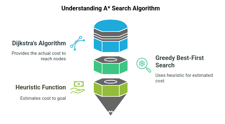
It combines the strengths of two powerful algorithms: Dijkstra’s algorithm and Greedy Breadth-First Search. It is powerful as it optimizes the estimated and actual cost of reaching a goal.
Post Graduate Program in Data Science with Generative AI: Applications to Business
Learn how to turn data into strategy in this UT Data Science and Business Analytics Course — now with a focus on Generative AI. Gain practical experience through 7 hands-on projects over a 7-month duration.
Graph Representation
In a*, the space is represented as a graph, where nodes represent positions or states and edges represent transitions between states. Edges are associated with costs or a given set of rules. The algorithm moves from the first node to the goal in consideration of the least-cost path.
Formula
A* Search Algorithm’s formula calculates the cost of reaching a particular node. The total cost of traversal is calculated as:
f(n)=g(n)+h(n)
Where:
- f(n) is the estimated total cost from the start node to the end goal via node n.
- g(n) is the actual cost from the start node to node n.
- h(n) is the heuristic cost (estimated cost) from node n to end node.
This heuristic cost or the guess of the remaining cost to the end goal is this algorithm's additional function, making it optimal amongst all pathfinding algorithms.
How does the A* Algorithm work?
A step-by-step implementation of this A* algorithm is given below:
- Initialization: The algorithm starts by placing the starting node in a priority queue. This priority queue, also known as an open list, contains all the nodes that have yet to be evaluated.
- Evaluation: This is the selection process in which the node with the lowest f(n) value from the queue is chosen for further operations.
- Expansion: The chosen node is evaluated by comparing it with its neighbours. For each neighbour, g(n) and h(n) values are calculated.
- Update: If a neighbour has a lower f(n) value than the recorded one, it is updated to the open list.
- Goal Check: The algorithm continues until the goal node is reached or the open list is empty, indicating no more path to traverse.
- Reconstruction: After finding the goal node, the algorithm reconstructs the path by tracing from the goal to the start node.
Python Implementation
The basic implementation of the A* algorithm in Python for a grid-based pathfinding problem is given below:
import heap
class Node:
def __init__(self, position, g, h):
self.position = position
self.g = g # Actual cost from start to this node
self.h = h # Heuristic cost to goal
self.f = g + h # Total cost
self.parent = None # To reconstruct the path
def __lt__(self, other):
return self.f < other.f
def a_star(grid, start, goal):
open_list = []
closed_list = set()
start_node = Node(start, 0, abs(start[0] - goal[0]) + abs(start[1] - goal[1])) # Manhattan distance as heuristic
heapq.heappush(open_list, start_node)
while open_list:
current_node = heapq.heappop(open_list)
if current_node.position == goal:
path = []
while current_node:
path.append(current_node.position)
current_node = current_node.parent
return path[::-1] # Return reversed path
closed_list.add(current_node.position)
# Check all 4 possible directions (up, down, left, right)
neighbors = [(0, 1), (1, 0), (0, -1), (-1, 0)]
for neighbor in neighbors:
neighbor_pos = (current_node.position[0] + neighbor[0], current_node.position[1] + neighbor[1])
if 0 <= neighbor_pos[0] < len(grid) and 0 <= neighbor_pos[1] < len(grid[0]) and grid[neighbor_pos[0]][neighbor_pos[1]] != 'X' and neighbor_pos not in closed_list:
g = current_node.g + 1
h = abs(neighbor_pos[0] - goal[0]) + abs(neighbor_pos[1] - goal[1])
neighbor_node = Node(neighbor_pos, g, h)
neighbor_node.parent = current_node
heapq.heappush(open_list, neighbor_node)
return None # No path found
# Example grid and usage
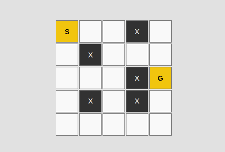
grid = [
['S', '1', '1', 'X', '1'],
['1', 'X', '1', '1', '1'],
['1', '1', '1', 'X', 'G']
]
start = (0, 0)
goal = (2, 4)
path = a_star(grid, start, goal)
print("Path found:", path)
Explanation of the above code:
Key Components
- Node Class: Represents a position in the grid with:
- position: Coordinates (x, y).
- g: Cost from start to this node.
- h: Heuristic cost to goal.
- f: Total cost (f = g + h).
- parent: Tracks the node's parent for path reconstruction.
- a_star Function:
- Input: Grid, start position, goal position.
- Process:
- Initializes a priority queue (open list) with the start node and a closed list to track processed nodes.
- Explores the current node's neighbours (up, down, left, right).
- Uses Manhattan distance as the heuristic (h).
- Adds valid neighbours to the open list, prioritizing nodes with the lowest f value.
- Output: Shortest path (list of coordinates) or None if no path exists.
Heuristics in A* Search
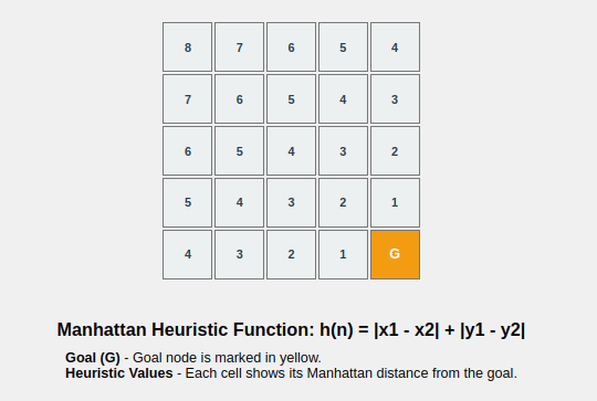
Heuristics play a very important role in the A* Search Algorithm as they are used to find the estimated cost of reaching the goal from a given node. The accuracy of the heuristic is directly related to the optimality of the path that A* finds.
Generally used heuristics are:
- Manhattan Distance: Used for grid-based pathfinding. Here, the diagonal moves are not allowed.
- Euclidean Distance: It is used for situations where diagonal moves are allowed.
- Chebyshev Distance: Used for grids where the cost of diagonal moves is the same as that of horizontal and vertical moves.
Applications of A* Search
As we have discussed above, A* Search Algorithm has many real-world applications, such as:
- Pathfinding in Games: A* algorithm is used in Artificial Intelligence Video Games where Non-player characters, commonly known as bots, find the shortest path throughout the game.
- Robotics: This algorithm also helps robots navigate through environments, avoiding obstacles.
- GPS Navigation: This algorithm is preferred to find the best and most efficient route between two points.
- Puzzle Solving: Puzzles where the target is to reach a goal from an initial position, such as 8-puzzle or sliding puzzles, take the help of A* Search Algorithm.
Advantages and disadvantages of A* Search Algorithm
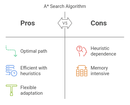
Advantages:
- Optimal: This algorithm is optimal as it guarantees the shortest possible path.
- Efficient: When an appropriate heuristic is used, it is faster than all other algorithms.
- Flexible: The algorithm is available to adapt to various types of graphs and different heuristics.
Disadvantages:
- Heuristic Dependent: The performance of this algorithm is heavily dependent on the choice of heuristics.
- Memory Intensive: This algorithm stores all the nodes in memory, which is not suitable for large graphs.
Conclusion
A* Search Algorithm is one of the best algorithms used in artificial intelligence and machine learning. It intelligently balances performance and efficiency. By combining the strengths of Dijkstra’s algorithm with greedy breadth-first search, a* produces optimal results.
The key role of heuristics in this algorithm is to allow it to calculate the estimated cost and prioritize paths.
Suggested: Free Artificial Intelligence Courses