Activation Functions in Neural Networks Explained

Activation functions play a crucial role in neural networks by determining whether a neuron should be activated or not. They introduce non-linearity, allowing networks to learn complex patterns. Without activation functions, a neural network would behave like a simple linear model, limiting its ability to solve real-world problems.

In this article, we’ll explore different types of activation functions, their applications, mathematical formulations, advantages, disadvantages, and how to choose the right one for your deep learning models.

What Are Activation Functions?

An activation function is a mathematical function applied to a neuron’s input to decide its output. It transforms the weighted sum of inputs into an output signal that is passed to the next layer in a neural network. The function’s primary objective is to introduce non-linearity into the network, enabling it to learn complex representations.

Without activation functions, a neural network could only model linear relationships, making it ineffective for solving non-trivial problems such as image classification, speech recognition, and natural language processing.

Why Are Activation Functions Necessary?

Neural networks consist of multiple layers where neurons process input signals and pass them to subsequent layers. Everything inside a neural network becomes a basic linear transformation when activation functions are removed, which renders the network unable to discover complex features.

Key reasons why activation functions are necessary:

• Introduce non-linearity: Real-world problems often involve complex, non-linear relationships. Activation functions enable neural networks to model these relationships.
• Enable hierarchical feature learning: Deep networks extract multiple levels of features from raw data, making them more powerful for pattern recognition.
• Prevent network collapse: Without activation functions, every layer would perform just a weighted sum, reducing the depth of the network into a single linear model.
• Improve convergence during training: Certain activation functions help improve gradient flow, ensuring faster and more stable learning.

Types of Activation Functions

1. Linear Activation Function

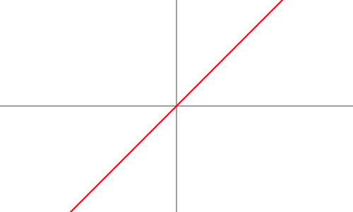
Formula: f(x) = ax

• The functioning produces an input value that has undergone scaling.
• The lack of non-linear elements prevents the network from fulfilling its complete learning capacity.
• Deep learning practitioners only infrequently use this activation function because it functions as a linear regression model.
• Use case: Often used in regression-based models where predicting continuous values is necessary.

2. Sigmoid Activation Function

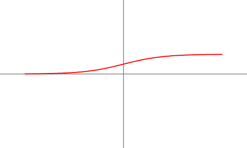
Formula: f(x) = 1 1 + e^-x

• Outputs values between 0 and 1.
• Useful for probability-based models like binary classification.
• Advantages: Smooth gradient, well-defined range, and interpretable output as probabilities.
• Drawbacks: Prone to the vanishing gradient problem, leading to slow learning in deep networks. It is also computationally expensive due to the exponentiation operation.

3. Tanh (Hyperbolic Tangent) Activation Function

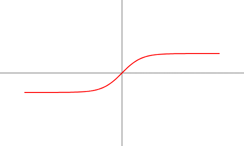
Formula: f(x) = e^x – e^-x e^x + e^-x

• Outputs values between -1 and 1.
• Centers the data around zero, helping in better gradient flow.
• Advantages: Scaled tanh activation offers enhanced gradient propagation since it operates from the zero-centered range.
• Drawbacks: The training of deep models becomes difficult because the deep networks experience reduced gradient propagation despite overcoming the sigmoid vanishing gradient problem.

4. ReLU (Rectified Linear Unit) Activation Function

Formula: f(x) = max(0, x)

• The most commonly used activation function in deep learning.
• Introduces non-linearity while avoiding the vanishing gradient problem.
• Advantages: Computationally efficient and prevents gradient saturation.
• Drawbacks: The implementation of “dying ReLU” results in dying neurons that stop learning because they become inactive when receiving negative inputs.

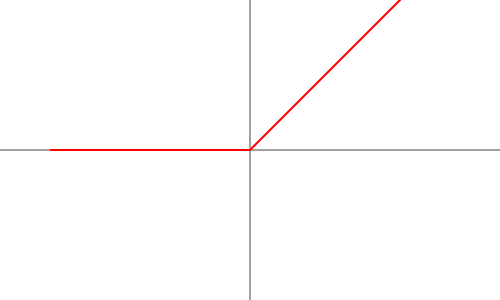
5. Leaky ReLU Activation Function

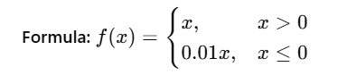
• A modified version of ReLU to allow small gradients for negative inputs.
• Helps to prevent dying neurons.
• Advantages: Maintains non-linearity while addressing ReLU’s limitation.
• Drawbacks: Choosing the best negative slope value is not always straightforward. Performance varies across different datasets.

6. ELU (Exponential Linear Unit) Activation Function

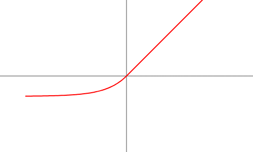
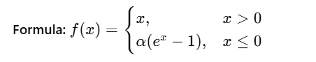
• The dying ReLU problem receives a solution because the activation function accepts small negative values.
• Advantages: Provides smooth gradient propagation and speeds up learning.
• Drawbacks: Computationally more expensive than ReLU, which can be an issue in large-scale applications.

7. Softmax Activation Function

• Used in multi-class classification problems.
• Converts logits into probabilities.
• Advantages: Ensures sum of probabilities equals 1, making it interpretable for classification tasks.
• Drawbacks: Computationally expensive and sensitive to outliers, as large input values can dominate the output.

Real-World Applications

Neural networks require activation functions as their main component to transform data into complex predictions that achieve accuracy. The applications of activation functions exist throughout real-world scenarios in the following implementations:

1. Image Recognition (ReLU & Softmax in CNNs)

Example: Face Recognition in Smartphones

• In facial recognition systems like Face ID, convolutional neural networks (CNNs) analyze facial features using ReLU activation in hidden layers to process pixel values efficiently.
• The final layer uses Softmax activation, which assigns probability scores to different faces to identify the correct person.

2. Natural Language Processing (NLP) (Tanh & Softmax in LSTMs & Transformers)

Example: Chatbots & Virtual Assistants

• Virtual assistants like Alexa, Siri, and Google Assistant use deep learning models with Tanh activation in LSTMs to understand sentence context.
• The last layer of language models uses Softmax activation to predict the most probable next word or response.

3. Healthcare – Medical Diagnosis (ReLU & Sigmoid in CNNs & DNNs)

Example: Cancer Detection from Medical Images

• In medical imaging (e.g., detecting tumors from MRI scans), CNNs with ReLU activation help extract important image features.
• The final layer uses Sigmoid activation to classify an image as either “cancerous” (1) or “non-cancerous” (0), helping doctors with early diagnosis.

4. Autonomous Vehicles (ReLU & Leaky ReLU in Deep Reinforcement Learning)

Example: Self-Driving Cars (Tesla Autopilot)

• Self-driving cars process real-time sensor data using deep learning.
• ReLU activation in neural networks helps recognize objects like pedestrians, road signs, and vehicles.
• Leaky ReLU activation prevents inactive neurons from making split-second driving decisions.

5. Fraud Detection (Sigmoid in Binary Classification Models)

Example: Credit Card Fraud Detection

• Banks use AI to detect fraudulent transactions by analyzing patterns in spending behavior.
• A binary classification neural network uses Sigmoid activation to classify whether a transaction is “fraud” (1) or “legitimate” (0).

Build a strong foundation in AI with this free Introduction to Neural Networks and Deep Learning course and learn key concepts from industry experts.

How to Choose the Right Activation Function?

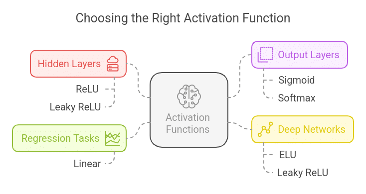
• For hidden layers, ReLU or Leaky ReLU is recommended due to efficient gradient propagation.
• For binary classification, Sigmoid is commonly used in the output layer.
• For multi-class classification, Softmax is the preferred choice.
• For deep networks: Consider using ELU or Leaky ReLU to avoid dead neurons.
• For regression tasks, Linear activation is used when predicting continuous values.

Practical Considerations

1. Computational Efficiency: Some activation functions, such as sigmoid and softmax, require expensive calculations, making them unsuitable for large networks.
2. Gradient Behavior: Activation functions should prevent the vanishing or exploding gradient problems to ensure stable training.
3. Network Depth: Deep networks require activation functions like ReLU that ensure proper gradient flow.
4. Interpretability: Because of their probability distribution output, the sigmoid, together with softmax, enables easier model interpretation in classification tasks.
5. Avoiding Dead Neurons: Choosing an activation function that prevents neurons from becoming inactive is crucial, especially in deeper networks.

Conclusion

Neural networks need activation functions to learn complex patterns in their systems. Activation functions determine both model performance as well as training efficiency in essential ways. Activation functions based on ReLU widely occur in hidden layers, but sigmoid and softmax work better for classification applications.

The awareness of activation function capabilities allows you to make strategic decisions about deep learning model construction.

Finding optimal activation functions per model design requires matching problem requirements with network constraints to create better-performing deep learning systems.

To build a strong foundation in neural network and deep learning concepts, enroll in our:

• Free Neural Network Course
• Free Deep Learning Courses

Frequently Asked Questions

1. Can I use multiple activation functions in a single neural network?

Yes. Different layers in a neural network can have different activation functions. For example, a CNN might use ReLU in hidden layers for feature extraction and Softmax in the output layer for classification.

Similarly, an RNN can use Tanh or ReLU for hidden states and Sigmoid for binary outputs.

2. Why is the Sigmoid function not widely used in deep networks?

The Sigmoid function suffers from the vanishing gradient problem, meaning that as inputs become large, their gradients become very small, slowing down learning. This makes it unsuitable for deep networks. Instead, ReLU and its variants (Leaky ReLU, ELU) are preferred in hidden layers.

3. What happens if I don’t use an activation function?

Without an activation function, all layers in the neural network will perform only linear transformations. No matter how many layers you add, the final output will still be a linear function of the input, making the network ineffective for solving complex problems like image recognition or natural language processing.

4. Which activation function is best for regression tasks?

The linear activation function serves regression problems since it demands continuous value estimations (e.g., house or stock prices) by acting on the output layer. Nonlinear ReLU activations remain necessary for hidden layers to use complex data connections properly.