It's easy for the human mind to distinguish between different types of fruits by noticing their color and shape.
But what if you ask a machine what type of fruit is in an image?
Ever wondered what the machine will answer?
This is where the concept of multiclass classification is introduced. You can detect the type of fruits or animals using a multiclass classifier or a machine learning model trained to classify an image into a particular class (or type of fruit/animal).
Let's learn what multiclass classification means.
What is multiclass classification?
Multiclass classification in Machine Learning classifies data into more than 2 classes or outputs using a set of features that belong to specific classes. Classification here means categorizing data and forming groups based on similarities or features.
The independent variables or features play a vital role in classifying our data in a dataset. Regarding multiclass classification, we have more than two classes in our dependent variable or output, as seen in Fig.1.
In Gmail, you will find that all incoming emails are segregated based on their content and importance. Some emails are of the utmost importance and go to the Primary tab, some go to Social for marketing content, and some go to the Spam folder if they are dangerous or clickbaity.
So, this classification of emails based on their content or their flagging based on specific words is an example of multiclass classification in machine learning.
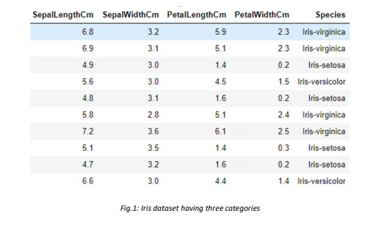
The above picture is taken from the Iris dataset which depicts that the target variable has three categories i.e., Virginica, setosa, and Versicolor, which are three species of Iris plant. We might use this dataset later, as an example of a conceptual understanding of multiclass classification.
MIT Data Science and Machine Learning Course
Unlock the power of data. Build hands-on data science and machine learning skills to drive innovation in your career.
Which classifiers do we use in multiclass classification? When do we use them?
We use many algorithms such as Naïve Bayes, Decision trees, SVM, Random forest classifier, KNN, and logistic regression for classification. But we might learn about only a few of them here because our motive is to understand multiclass classification. So, using a few algorithms we will try to cover almost all the relevant concepts related to multiclass classification.
1. Naive Bayes
Naive Bayes is a parametric algorithm that requires a fixed set of parameters or assumptions to simplify the machine's learning process. In parametric algorithms, the number of parameters used is independent of the size of the training data.
Naïve Bayes Assumption:
- It assumes that the features of a dataset are entirely independent of each other. But it is generally not true. That is why we also call it a 'naïve' algorithm.
How it works?
It is a classification model based on conditional probability that uses the Bayes theorem to predict the class of unknown datasets. This model is mostly used for large datasets as it is easy to build and fast for both training and prediction. Moreover, without hyperparameter tuning, it can give better results than other algorithms.
Naïve Bayes can also be an extremely good text classifier as it performs well, such as in the spam ham dataset.
Bayes theorem is stated as-

- By P (A|B), we are trying to find the probability of event A given that event B is true. It is also known as posterior probability.
- Event B is known as evidence.
- P (A) is called priori of A which means it is probability of event before evidence is seen.
- P (B|A) is known as conditional probability or likelihood.
Note: Naïve Bayes’ is linear classifier which might not be suitable to classes that are not linearly separated in a dataset. Let us look at the figure below:
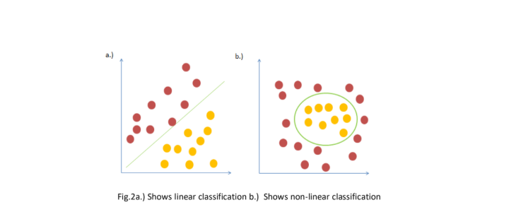
As can be seen in Fig.2b, Classifiers such as KNN can be used for non-linear classification instead of Naïve Bayes classifier.
Advantages
- It is beneficial in cases involving large datasets and many dimensions
- One of the most efficient algorithm in terms of training when you have limited data and very fast when testing
- Works well for multiclass classification which involves categorical variables
Disadvantages
- It is naive in terms of assuming every feature to be independent of one another
- Independence of every feature is not possible in real life hence some dependent features influence the output
- Might not generalize well on unseen data as zero is assigned as probability
2. KNN (K-nearest neighbours)
KNN is a supervised machine learning algorithm that can be used to solve both classification and regression problems. It is one of the simplest yet powerful algorithms. It does not learn a discriminative function from the training data but memorizes it instead. For this reason, it is also known as a lazy algorithm.
How it works?
The K-nearest neighbor algorithm forms a majority vote between the K most similar instances, and it uses a distance metric between the two data points to define them as identical. The most popular choice is Euclidean distance, which is written as:

K in KNN is the hyperparameter we can choose to get the best possible fit for the dataset. Suppose we keep the smallest value for K, i.e., K=1. In that case, the model will show low bias but high variance because our model will be overfitted.
A more significant value for K, k=10, will surely smoothen our decision boundary, meaning low variance but high bias. So, we always go for a trade-off between the bias and variance, known as a bias-variance trade-off.
Let us understand more about it by looking at its advantages and disadvantages:
Advantages-
- KNN makes no assumptions about the distribution of classes i.e. it is a non-parametric classifier
- It is one of the methods that can be widely used in multiclass classification
- It does not get impacted by the outliers
- This classifier is easy to use and implement
Disadvantages-
- K value is difficult to find as it must work well with test data also, not only with the training data
- It is a lazy algorithm as it does not make any models
- It is computationally extensive because it measures distance with each data point
Decision Trees
As the name suggests, the decision tree is a tree-like structure of decisions made based on some conditional statements. This is one of the most used supervised learning methods in classification problems because of their high accuracy, stability, and easy interpretation. They can map linear as well as non-linear relationships in a good way.
Let us look at the figure below, Fig.3, where we have used adult census income dataset with two independent variables and one dependent variable. Our target or dependent variable is income, which has binary classes i.e, <=50K or >50K.
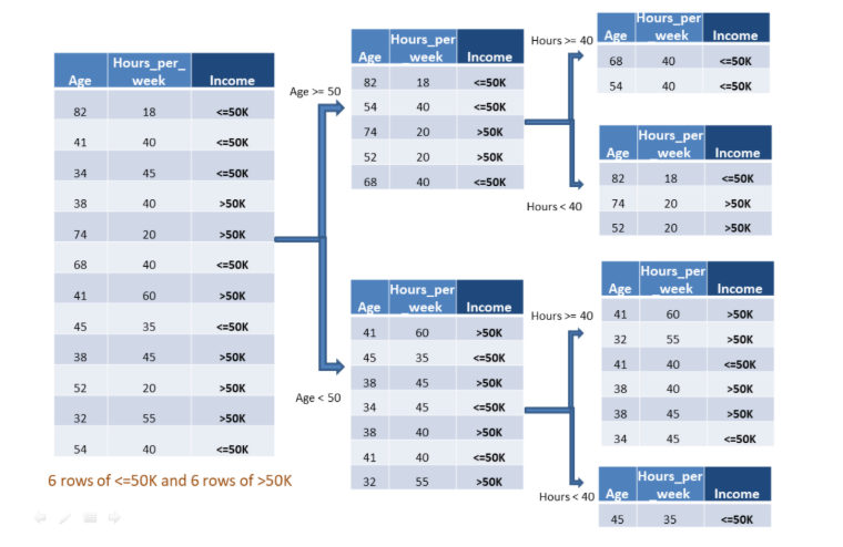
We can see that the algorithm works based on some conditions, such as Age <50 and Hours>=40, to further split into two buckets for reaching towards homogeneity. Similarly, we can move ahead for multiclass classification problem datasets, such as Iris data.
Now a question arises in our mind. How should we decide which column to take first and what is the threshold for splitting? For splitting a node and deciding threshold for splitting, we use entropy or Gini index as measures of impurity of a node. We aim to maximize the purity or homogeneity on each split, as we saw in Fig.2.
Post Graduate Program in Artificial Intelligence for Leaders
Turn insights into action—use AI to make faster decisions, optimize teams, and lead digital transformation.
What is Entropy?
Entropy or Shannon entropy is the measure of uncertainty, which has a similar sense as in thermodynamics. By entropy, we talk about a lack of information. To understand better, let us suppose we have a bag full of red and green balls.
Scenario1: 5 red balls and 5 green balls.

If you are asked to take one ball out of it then what is the probability that the ball will be green colour ball?
Here we all know there will have 50% chances that the ball we pick will be green.
Scenario2: 1 red and 9 green balls
Here the chances of red ball are minimum and we are certain enough that the ball we pick will be green because of its 9/10 probability.
Scenario3: 0 red and 10 green balls
In this case, we are very certain that the ball we pick is of green colour.
In the second and third scenario, there is high certainty of green ball in our first pick or we can say there is less entropy. But in the first scenario there is high uncertainty or high entropy.
Entropy ∝ Uncertainty
Formula for entropy:

Where p(i) is probability of an element/class ‘i’ in the data
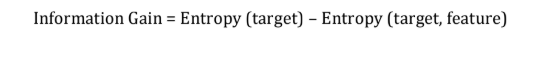
After finding entropy we find Information gain which is written as below:
What is Gini Index?
Gini is another useful metric to decide splitting in decision trees.
Gini Index formula:

Where p(i) is probability of an element/class ‘i’ in the data.
We have always seen logistic regression is a supervised classification algorithm being used in binary classification problems. But here, we will learn how we can extend this algorithm for classifying multiclass data.
In binary, we have 0 or 1 as our classes, and the threshold for a balanced binary classification dataset is generally 0.5.
Whereas, in multiclass, there can be 3 balanced classes for which we require 2 threshold values which can be, 0.33 and 0.66.
But a question arises, by using what method do we calculate threshold and approach multiclass classification?
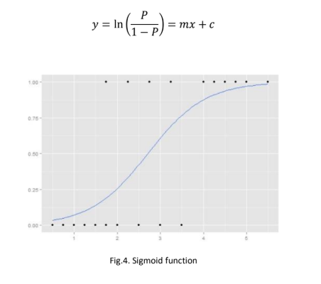
So let’s first see a general formula that we use for the logistic regression curve:
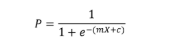
Where P is the probability of the event occurring and the above equation derives from here:
There are two ways to approach this kind of a problem. They are explained as below:
One vs. Rest (OvR)– Here, one class is considered as positive, and rest all are taken as negatives, and then we generate n-classifiers. Let us suppose there are 3 classes in a dataset, therefore in this approach, it trains 3-classifiers by taking one class at a time as positive and rest two classes as negative. Now, each classifier predicts the probability of a particular class and the class with the highest probability is the answer.
One vs. One (OvO)– In this approach, n ∗ (n − 1)⁄2 binary classifier models are generated. Here each classifier predicts one class label. Once we input test data to the classifier, the class which has been predicted the most is chosen as the answer.
Confusion Matrix in Multi-class Classification
A confusion matrix is a table used in every classification problem to describe the performance of a model on test data.
As we know about the confusion matrix in binary classification, we can also in multiclass classification
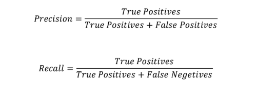
Let's take an example to understand how we can find precision and recall accuracy using a confusion matrix in multiclass classification.
Finding precision and recall from above Table 1:
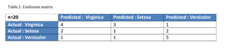
Precision for the Virginica class is the number of correctly predicted virginica species out of all the predicted virginica species, which is 4/7 = 57.1%. This means that only 4/7 of the species our predictor classifies as Virginica are virginica. Similarly, we can find for other species, i.e., for Setosa and Versicolor, precision is 20% and 62.5%, respectively.
Recall for the Virginica class is the number of correctly predicted virginica species out of actual virginica species, which is 50%. This means that our classifier classified half of the virginica species as virginica. Similarly, we can find for other species, i.e., for Setosa and Versicolor, recall is 20% and 71.4%, respectively.
Multiclass Vs Multi-label
People often get confused between multiclass and multi-label classification. But these two terms are very different and cannot be used interchangeably. We have already understood what multiclass is all about. Let’s discuss in brief how multi-label is different from multiclass.
Multi-label refers to a data point that may belong to more than one class. For example, you wish to watch a movie with your friends but you have a different choice of genres that you all enjoy. Some of your friends like comedy and others are more into action and thrill. Therefore, you search for a movie that fulfills both the requirements and here, your movie is supposed to have multiple labels. Whereas, in multiclass or binary classification, your data point can belong to only a single class. Some more examples of the multi-label dataset could be protein classification in the human body, or music categorization according to genres. It can also one of the concepts highly used in photo classification.
I hope this article has provided you with some fair conceptual knowledge. Don't stop here, remember that there are many more ways to classify your data. All that is important is how you polish your basics to create and implement more algorithms. Let us conclude by looking at what Professor Pedro Domingos said-
“Machine learning will not single-handedly determine the future, any more than any other technology; it’s what we decide to do with it that counts, and now you have the tools to decide.”
Our Machine Learning Courses
Explore our Machine Learning and AI courses, designed for comprehensive learning and skill development.
| Program Name | Duration |
|---|---|
| MIT No code AI and Machine Learning Course | 12 Weeks |
| MIT Data Science and Machine Learning Course | 12 Weeks |
| Data Science and Machine Learning Course | 12 Weeks |