How to Use the HLOOKUP Function in Excel?

Looking for an easy way to fetch your data in Excel? 

The HLOOKUP function enables you to quickly and easily locate data in rows by searching horizontally. 

Whether you are looking at sales, prices, or any other metrics, the formula can retrieve exact information from a table.

In this tutorial, we’ll review how the HLOOKUP function works, use real examples, and explain all the steps to become an Excel expert.

What does HLOOKUP do in Excel?

The HLOOKUP function in Excel helps you search in the top row, then gives you a value from another row in the same column.

You can use this function most effectively if your data is gathered with headers in the first row and data entries below.

HLOOKUP Syntax:

=HLOOKUP(lookup_value, table_array, row_index_num, [range_lookup])

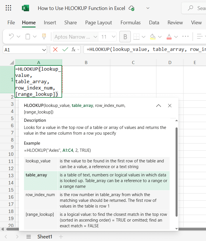
Explanation of Each Argument:

1. lookup_value

• The value you want to find in the first row of your table or data range.
• This can be a number, text, cell reference, or even a formula.
• Example: "Q2" or B1.

2. table_array

• The range of cells that contains the data you want to search through.
• The first row of this range is where HLOOKUP will look for the lookup_value.
• Example: A1:D3.

3. row_index_num

• The row number within your selected table where the data you want to retrieve is located.
• For example, 2 means the result will come from the second row of the table_array.
• Must be greater than or equal to 1 and less than or equal to the total number of rows in the table_array.

Note: If you type 1, HLOOKUP will return the header itself (the first row). Since you usually want the data below the header, your Row Index Number will almost always be 2 or higher.

4. [range_lookup] (Optional)

• A logical value:

• TRUE = Approximate match (default)
• FALSE = Exact match

• If omitted, Excel assumes TRUE.
• Important: When using TRUE, the data in the first row must be sorted in ascending order.

Step-by-Step Guide: How to Use HLOOKUP in Excel (with an Example)

Suppose you want to check the sales numbers from a certain quarter in your quarterly sales data.

Step 1: Enter Your Dataset

Open Excel and input the following data starting from cell A1:

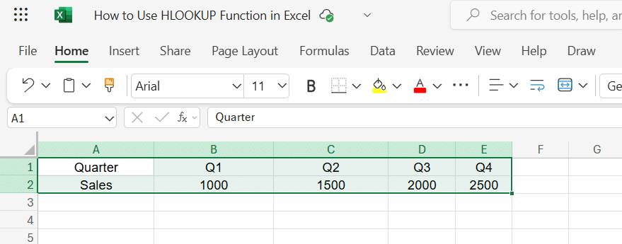
You should have this dataset in the range A1:E2, where:

• Row 1 contains quarters (Q1 to Q4).
• Row 2 contains the corresponding sales figures.

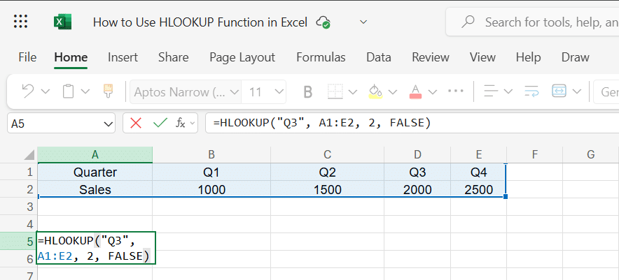
Step 2: Choose a Cell for the Formula

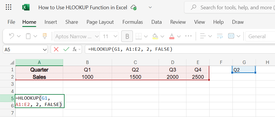
Click on a new cell, for example, A5, where you want to display the result of the HLOOKUP function.

Step 3: Enter the HLOOKUP Formula

Now, enter the following formula in cell A5:

=HLOOKUP("Q3", A1:E2, 2, FALSE)

Explanation of the formula:

• "Q3": The value to look for in the top row.
• A1:E2: The range containing your data.
• 2: The row number containing the answers (Sales).
• FALSE: Ensures Excel looks for "Q3" exactly, not a partial match.

Pro Tip: Locking Your Table

In this example, we used the range A1:E2. 

However, in professional reports, it is best practice to "lock" your table range by adding dollar signs ($), like this: $A$1:$E$2.

This is called an Absolute Reference. 

It ensures that if you copy and paste this formula to another cell, the reference to your data table stays fixed and doesn't move, preventing errors.

To keep the examples below simple and easy to read, we have skipped the dollar signs. You only need them if you plan to copy the formula to other cells.

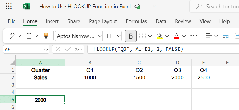
Step 4: Press Enter

Once you press Enter, the result will display as: 2000, the sales figure for Q3.

Step 5: Try a Cell Reference Instead of a Direct Value

To make the formula more dynamic, replace "Q3" with a cell reference.

1. In cell G1, type: Q2
2. In cell A5, use this formula:

The answer will be 1500

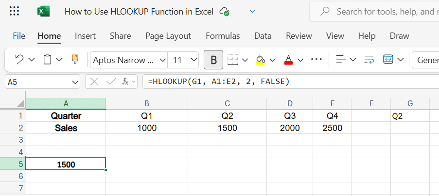
Now, the lookup value will depend on the value in G1. Try changing G1 to Q4 and see if the result updates to 2500.

Step 6: What Happens with an Incorrect or Missing Value?

Try entering an invalid quarter in G1, like Q5, with the formula =HLOOKUP(G1, A1:E2, 2, FALSE) and it will return: #N/A

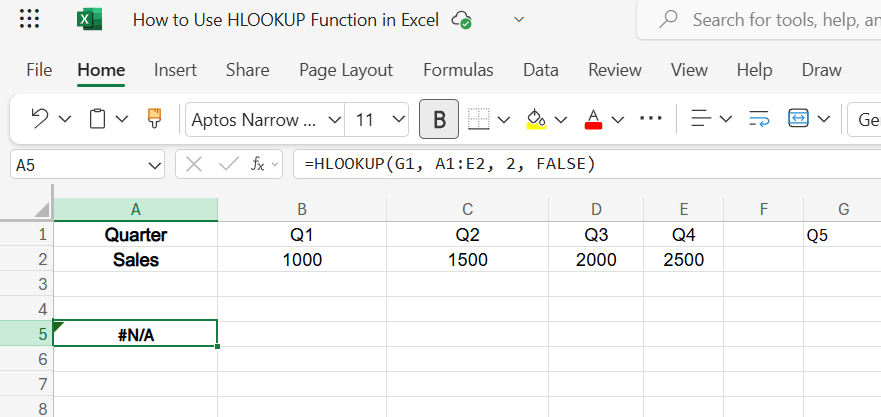
This indicates that the exact match couldn’t be found in the first row.

Summary:

• HLOOKUP is great for horizontally structured data.
• Always define a clear lookup row (first row in the range).
• Use FALSE for an exact match to avoid unexpected results.
• Replace static values with cell references for dynamic lookup.

More Practical Examples of HLOOKUP

Example 1: Simple Exact Match to Find a Student’s Score

Scenario: 

You have a table of students' scores in different subjects. You want to look up the score of a specific student in a particular subject.

Sample Data (starting at cell A1)

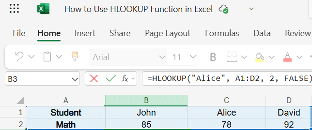
Objective: Find Alice’s score in Math.

Formula:

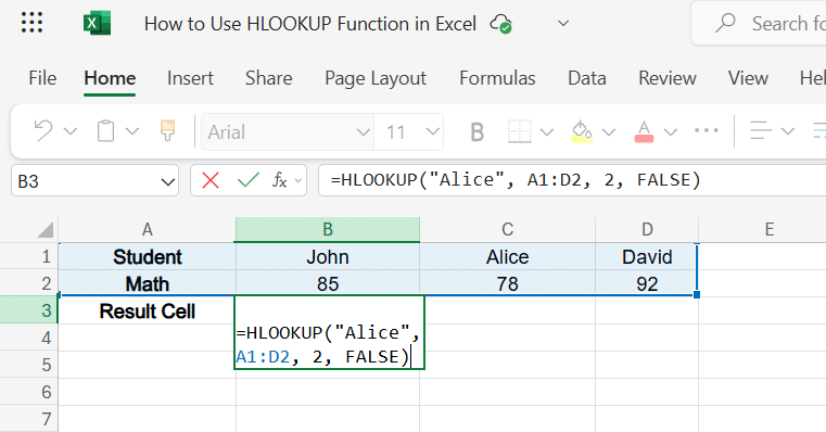
Explanation:

• "Alice" is the student you want to look up.
• A1:D2 is the table containing names and scores.
• 2 indicates you want the value from the second row (Math scores).
• FALSE enforces an exact match.

Result: 78

Example 2: Using Wildcards for Partial Text Matches

Scenario: 

You want to find a student's math score, but you only know their name starts with "Da" (e.g., David).

You can use a wildcard character (the asterisk *) to tell Excel to look for any text that follows Da":*.

The Formula:
To find the score for the student starting with "Da", enter this formula:

=HLOOKUP("Da*", A1:D2, 2, FALSE)

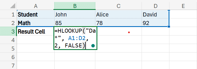
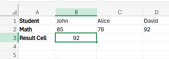
Result: 92 (This is David's score).

Explanation:

• "Da"*: The asterisk (*) is a wildcard that represents any number of characters. Excel reads this as "Find a cell that starts with 'Da' and has anything (or nothing) after it."

• A1:D2: The range containing the names and scores.

• 2: You want the data from the second row (the scores).

• FALSE: Crucial Step.
  You must use FALSE (Exact Match) for wildcards to work correctly. 

If you use TRUE, Excel will treat the wildcard as a standard character or try to find the closest sorted value, which will give you an error or the wrong result.

Note: 

HLOOKUP searches from left to right and stops at the first match it finds. 

If you have a student named "Daniel" listed before "David," the formula will return Daniel's score because he also matches "Da*".

Now that we've covered exact and partial matches, let's look at how to handle scenarios where an exact match isn't required.

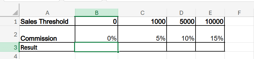
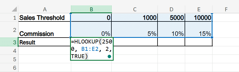
Example 3: Calculating Sales Commissions (Approximate Match)

Scenario:

You want to assign a commission rate to salespeople based on how much they sell. The rates work in "tiers" or brackets:

• $0 - $999 gets 0%
• $1,000 - $4,999 gets 5%
• $5,000 - $9,999 gets 10%
• $10,000+ gets 15%

Step 1: 

Set up your Data (Must be Sorted)

For an approximate match to work, the first row must be sorted from smallest to largest.

Step 2:
A salesperson made $2,500 in sales. You want to find their rate and to get that enter this formula:

=HLOOKUP(2500, B1:E2, 2, TRUE)

Step 4: The result will be 5%.

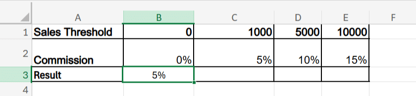
The Logic:

1. The Rule: When TRUE is used, Excel searches for the largest value that is less than or equal to your lookup value (2500).

2. Compare: Excel compares 2500 against the sorted header row. It determines that 2500 is greater than 1000, but smaller than the next threshold (5000).

3. Match: Because it hasn't reached 5000 yet, Excel falls back to the previous largest match, which is 1000, and returns the commission rate associated with that column (5%).

4. What if the data isn't sorted?
If your sales thresholds were mixed up (e.g., 5000, then 1000, then 0), HLOOKUP would get confused and likely return a wrong commission rate or an error. This is why ascending order is mandatory for approximate matches.

Rule for Learners

If you use TRUE (or leave the last part blank), you must sort your first row in ascending order (0, 1000, 5000). If the row is mixed up (e.g., 5000, 0, 1000), Excel will give you a wrong answer or an error.

Common Mistakes and Troubleshooting in HLOOKUP

1. Mixing Up Row and Column Orientation

Issue:
Users often confuse HLOOKUP with VLOOKUP. HLOOKUP searches horizontally in the first row of a table, not vertically.

Example Mistake: Trying to search for a value in the first column using HLOOKUP:

=HLOOKUP("Math", A1:A5, 2, FALSE) → Incorrect (should be VLOOKUP)

Fix:
Ensure your lookup value is in the first row, and the data to be returned is in rows below it.

2. Forgetting to Use FALSE for Exact Matches

Issue:
By default, HLOOKUP uses approximate match (TRUE) if the fourth argument is omitted, which can return inaccurate results.

Example Mistake:

=HLOOKUP("Alice", A1:D2, 2) → Might return the wrong value

Fix:
Always use FALSE for an exact match unless you're intentionally using an approximate match:

=HLOOKUP("Alice", A1:D2, 2, FALSE)

3. Not Sorting the First Row When Using Approximate Match

Issue:
When using TRUE (Approximate Match), HLOOKUP assumes your data is organized from smallest to largest. 

It stops at the value closest to your lookup value without going over. If the row isn't sorted, HLOOKUP might return the wrong data, either too early or too late.

Example Mistake:

=HLOOKUP(82, A1:D2, 2, TRUE) → Incorrect if A1:D1 isn’t sorted numerically

Fix:
Always sort the first row in ascending order (smallest to largest) when using an approximate match (TRUE).

• Sort: 0, 50, 70, 90
• Then use: =HLOOKUP(82, A1:D2, 2, TRUE)
• Result: Excel will stop at 70 (because 82 is larger than 70 but smaller than 90) and return the corresponding value.

4. Dealing with #N/A Errors and How to Resolve Them

Issue:
HLOOKUP returns #N/A when:

• The lookup value isn’t found.
• You use FALSE, but the exact match doesn’t exist.
• You reference a row number that doesn’t exist in the table range.

Fixes:

• Double-check spelling or spacing of the lookup value.
• Make sure the row_index_num is within the table range.
• Use IFERROR() to handle errors gracefully:

=IFERROR(HLOOKUP("David", A1:D2, 2, FALSE), "Not Found")

By keeping these common issues in check, you'll ensure your HLOOKUP formulas return accurate and reliable results.

HLOOKUP vs. VLOOKUP: When to Use Each

Feature / Criteria	HLOOKUP	VLOOKUP
Function Name	Horizontal Lookup	Vertical Lookup
Data Orientation	Works across rows (horizontal layout)	Works down columns (vertical layout)
Lookup Direction	Searches the first row and returns a value in the same column from a specified row number.	Searches the first column and returns from the right
Syntax	=HLOOKUP(lookup_value, table_array, row_index_num, [range_lookup])	=VLOOKUP(lookup_value, table_array, col_index_num, [range_lookup])
Use Case Example	Finding marks of subjects listed across a row	Finding employee details listed in a column
Index Parameter	row_index_num	col_index_num
Data Requirement	Lookup value must be in the first row of the range	Lookup value must be in the first column of the range
Ease of Use	Less commonly used; suitable for wide tables	More commonly used, suitable for tall tables
Common Mistake	Using it for column-wise data	Using it for row-wise data
Example	=HLOOKUP("Math", A1:E3, 2, FALSE)	=VLOOKUP("John", A1:C5, 2, FALSE)

Learn: How To Use the VLookup Function in Excel?

Important: Look at where your headers (titles) are located:

• Headers on Top? Then use HLOOKUP (Horizontal)
• Headers on the Left? Then use VLOOKUP (Vertical)

The HLOOKUP function is a quick way to find information stored in rows, helping you locate the data you need without manual searching. 

To improve your overall Excel skills and learn how to use formulas like HLOOKUP more confidently, Great Learning’s Data Analytics in Excel course offers practical, step-by-step training that helps you work smarter with data in any role.