This guide provides 27 practical SQL query examples to help you master data analysis. We will start from basic data retrieval with SELECT to advanced analytical techniques using window functions and CTEs.
This article focuses specifically on querying - the method of asking questions to get answers from your data. If you need a foundational overview of all SQL command types (like DDL for creating tables or DCL for permissions) first, see our complete guide to SQL Commands.
We'll use two simple tables for most examples: employees and departments.
employees table:
| employee_id | first_name | last_name | salary | department_id | hire_date |
|---|---|---|---|---|---|
| 1 | John | Smith | 60000 | 1 | 2022-01-15 |
| 2 | Jane | Doe | 75000 | 1 | 2021-03-20 |
| 3 | Peter | Jones | 90000 | 2 | 2020-05-10 |
| 4 | Mary | Williams | 80000 | 2 | 2021-08-01 |
| 5 | David | Brown | 65000 | 3 | 2023-01-05 |
| 6 | null | Davis | 55000 | 3 | 2023-02-12 |
departments table:
| department_id | department_name |
|---|---|
| 1 | Engineering |
| 2 | Sales |
| 3 | Marketing |
| 4 | HR |
Master SQL and Database management with this SQL course: Practical training with guided projects, AI support, and expert instructors.
The Basics: Data Retrieval
These are the basic queries you'll use every single day. Don't just learn them, know them.
1. SELECT *
What it does: Selects all columns from a table.
Example:
SELECT * FROM employees;
Explanation: This query returns every single row and column from the employees table. Use it to get a quick look at your data.
2. SELECT [specific columns]
What it does: Selects only the columns you specify. More efficient than SELECT *.
Example:
SELECT first_name, last_name, salary FROM employees;
Explanation: Returns only the first_name, last_name, and salary for all employees.
3. WHERE
What it does: Filters records based on a condition.
Example:
SELECT * FROM employees WHERE salary > 70000;
Explanation: This shows all information for employees earning more than 70,000.
4. AND / OR
What it does: Combines multiple conditions in a WHERE clause.
Example:
SELECT * FROM employees WHERE salary > 70000 AND department_id = 2;
Explanation: Retrieves employees who are in department 2 AND have a salary over 70,000.
5. ORDER BY
What it does: Sorts the results. The default is ascending (ASC).
Example:
SELECT first_name, salary FROM employees ORDER BY salary DESC;
Explanation: Displays employee first names and salaries, sorted from highest salary to lowest.
6. LIMIT
What it does: Restricts the number of rows returned.
Example:
SELECT * FROM employees ORDER BY hire_date DESC LIMIT 3;
Explanation: Gets the top 3 most recently hired employees.
7. DISTINCT
What it does: Returns only unique values.
Example:
SELECT DISTINCT department_id FROM employees;
Explanation: Shows a list of unique department_ids that have employees, which would be 1, 2, and 3.
8. LIKE
What it does: Used in a WHERE clause to search for a specific pattern in a column.
Example:
SELECT first_name, last_name FROM employees WHERE last_name LIKE 'J%';
Explanation: Finds all employees whose last name starts with 'J'. The % is a wildcard.
9. IS NULL / IS NOT NULL
What it does: Checks for empty values.
Example:
SELECT * FROM employees WHERE first_name IS NULL;
Explanation: Retrieves rows where the first_name has not been entered, like employee_id 6.
Medium Level Queries: Joins and Aggregations
This is where you start combining and analyzing data. Master these, and you're hireable.
10. INNER JOIN
What it does: Combines rows from two or more tables based on a related column. Returns only matching rows.
Example:
SELECT e.first_name, e.last_name, d.department_name
FROM employees e
INNER JOIN departments d ON e.department_id = d.department_id;
Explanation: This query lists each employee and their corresponding department name. The HR department won't show up because no employee is assigned to it.
11. LEFT JOIN
What it does: Returns all records from the left table (employees), and the matched records from the right table (departments).
Example:
SELECT e.first_name, d.department_name
FROM employees e
LEFT JOIN departments d ON e.department_id = d.department_id;
Explanation: Shows all employees and their department. If an employee had a department_id that didn't exist in departments, their department_name would be NULL.
12. RIGHT JOIN
What it does: Returns all records from the right table (departments), and the matched records from the left.
Example:
SELECT e.first_name, d.department_name
FROM employees e
RIGHT JOIN departments d ON e.department_id = d.department_id;
Explanation: This will list all departments and the employees in them. The HR department will appear with a NULL first_name because it has no employees.
Also Read: SQL Joins - Inner, Left, Right & Full Join
13. COUNT()
What it does: An aggregate function that counts the number of rows.
Example:
SELECT COUNT(*) FROM employees;
Explanation: Returns the total number of employees, which is 6.
14. SUM()
What it does: Calculates the total sum of a numeric column.
Example:
SELECT SUM(salary) FROM employees WHERE department_id = 1;
Explanation: Calculates the total salary for all employees in the Engineering department (60000 + 75000).
15. AVG()
What it does: Calculates the average value of a numeric column.
Example:
SELECT AVG(salary) FROM employees;
Explanation: Gives the average salary of all employees.
16. GROUP BY
What it does: Groups rows that have the same values into summary rows. Often used with aggregate functions.
Example:
SELECT department_id, COUNT(employee_id) as num_employees
FROM employees
GROUP BY department_id;
Explanation: Shows how many employees are in each department.
17. HAVING
What it does: Filters groups based on a condition after GROUP BY. WHERE filters rows before grouping.
Example:
SELECT d.department_name, AVG(e.salary) as avg_salary
FROM employees e
JOIN departments d ON e.department_id = d.department_id
GROUP BY d.department_name
HAVING AVG(e.salary) > 70000;
Explanation: This query shows departments where the average salary is greater than 70,000.
18. CASE
What it does: Adds if-then-else logic to your queries.
Example:
SELECT first_name, salary,
    CASE
        WHEN salary > 85000 THEN 'High Earner'
        WHEN salary > 70000 THEN 'Mid Earner'
        ELSE 'Standard Earner'
    END as salary_bracket
FROM employees;
Explanation: Creates a new column salary_bracket and categorizes each employee based on their salary.
19. Subquery (or Inner Query)
What it does: A query nested inside another query.
Example:
SELECT first_name, last_name
FROM employees
WHERE department_id IN (SELECT department_id FROM departments WHERE department_name = 'Sales');
Explanation: Gets the names of all employees who work in the 'Sales' department. The inner query finds the department_id for Sales first.
Advanced SQL Queries: Window Functions and CTEs
If you can use these fluently, you're not a junior anymore. These are for complex analysis.
20. Common Table Expression (CTE)
What it does: Creates a temporary, named result set that you can reference within your main query.
Example:
WITH HighSalaries AS (
    SELECT employee_id, first_name, salary
    FROM employees
    WHERE salary > 75000
)
SELECT * FROM HighSalaries;
Explanation: The WITH clause defines a temporary table HighSalaries, which is then queried. It's cleaner than a subquery for complex logic.
21. ROW_NUMBER()
What it does: A window function that assigns a unique number to each row within a partition.
Example:
SELECT
    first_name,
    department_name,
    salary,
    ROW_NUMBER() OVER(PARTITION BY department_name ORDER BY salary DESC) as rank_in_dept
FROM employees e
JOIN departments d ON e.department_id = d.department_id;
Explanation: This ranks employees within each department based on salary. The highest salary in each department gets rank 1.
22. RANK() & DENSE_RANK()
What it does: Ranks rows within a partition. RANK() will skip ranks after a tie (e.g., 1, 2, 2, 4), while DENSE_RANK() will not (e.g., 1, 2, 2, 3).
Example:
SELECT
    first_name,
    salary,
    RANK() OVER(ORDER BY salary DESC) as salary_rank
FROM employees;
Explanation: Assigns a rank to each employee based on their overall salary.
23. LAG() & LEAD()
What it does: Accesses data from a previous row (LAG) or a subsequent row (LEAD) without a self-join.
Example: (Assume a table sales with sale_date and sale_amount)
SELECT
    sale_date,
    sale_amount,
    LAG(sale_amount, 1, 0) OVER(ORDER BY sale_date) as previous_day_sales
FROM sales;
Explanation: Shows each day's sales next to the previous day's sales, making day-over-day comparisons easy.
24. Moving Average
What it does: Calculates averages over a specific window of rows.
Example:
SELECT
    sale_date,
    sale_amount,
    AVG(sale_amount) OVER(ORDER BY sale_date ROWS BETWEEN 2 PRECEDING AND CURRENT ROW) as three_day_moving_avg
FROM sales;
Explanation: For each day, it calculates the average sales of that day and the two preceding days.
25. PIVOT (Conditional Aggregation)
What it does: Rotates a table by turning unique values from one column into multiple columns.
Example: (using CASE for general compatibility)
SELECT
    department_id,
    COUNT(CASE WHEN salary > 70000 THEN 1 END) as high_earners,
    COUNT(CASE WHEN salary <= 70000 THEN 1 END) as standard_earners
FROM employees
GROUP BY department_id;
Explanation: Creates a report showing the count of high vs. standard earners for each department.
26. Self Join
What it does: Joining a table to itself to compare rows within the same table.
Example: Find employees who were hired on the same day.
SELECT e1.first_name, e1.last_name, e2.first_name, e2.last_name, e1.hire_date
FROM employees e1
JOIN employees e2 ON e1.hire_date = e2.hire_date AND e1.employee_id > e2.employee_id;
Explanation: Compares every employee record (e1) with every other employee record (e2) to find matches on hire_date. e1.employee_id > e2.employee_id prevents duplicates and self-matching.
27. UNION / UNION ALL
What it does: Combines the result set of two or more SELECT statements. UNION removes duplicates, UNION ALL includes all records.
Example:
SELECT first_name, last_name FROM employees WHERE department_id = 1
UNION
SELECT first_name, last_name FROM employees WHERE department_id = 2;
Explanation: Creates a single list of all employees from departments 1 and 2.
Best Practices for Writing Effective Queries
- Write Clearly: Use short names (aliases) for tables in joins (like
efor employees). Make your code easy to read by using spaces and putting parts on new lines. Add comments (--at the start of a line) to explain tricky parts. - Make Them Fast: Use
CREATE INDEXon columns you often filter or join on. Only select the columns you actually need; don't just useSELECT *. Look at the "query plan" to see how the database runs your query and where it's slow. - Avoid Problems: Remember that
NULLis tricky; useIS NULLorIS NOT NULLto check for it. Test your queries on a small amount of data first. Double-check yourJOINconditions to make sure you are linking tables correctly.
Conclusion
SQL queries are powerful tools. They let you get, analyze, and understand the data in your databases.
We've looked at many types of queries, from simple selections to complex joins and aggregations.
What should you do next? Practice! Find some sample databases online (like AdventureWorks or Chinook) and try running these queries yourself.
You can use this Online SQL Compiler Tool to easily test queries.
Keep trying and exploring. The more you write and run queries, the better you will become at extracting insights from your data!