- What is Conditional Formatting in Excel?
- Why Use Conditional Formatting?
- How to Use Conditional Formatting in Excel
- Types of Conditional Formatting Rules in Excel
- Examples of Conditional Formatting in Action
- How do I use a Formula in Conditional Formatting?
- Common Issues and How to Fix Them
- Conclusion + Final Tips
- Frequently Asked Questions (FAQs)
What is Conditional Formatting in Excel?
Conditional formatting in Excel is a powerful feature that allows users to automatically change the appearance of cells based on the data they contain. Conditional formatting can reveal some of the most important patterns and trends, no matter whether you are tracking project deadlines, budgets, or analyzing sales performance, with a minimum amount of effort.
For example, you might use conditional formatting to:
- Highlight sales figures above a certain target in green
- Mark overdue tasks in red
- Add a color scale to show low-to-high performance values
- Use data bars to visually compare quantities across rows
These visual enhancements help make raw data easier to scan and interpret. Instead of hunting through rows of numbers, key insights jump out immediately.
Learn Excel the smart way! Our course teaches you all the essential tools and techniques to master spreadsheets, from formulas to charts, and improve your workflow in every task you do.
Why Use Conditional Formatting?
- Improves readability: Color cues and visual elements make dense information easier to scan.
- Highlights critical data: Immediately identify values that satisfy certain criteria, e.g. large-scale sales, low stocks, or late delivery.
- Aids decision-making: You are able to prioritize the important data using clear visuals; more quickly and more accurately.
Conditional formatting is just one piece of the puzzle, learn how to do full-scale analysis in Excel with this course: Data Analytics with Excel.
How to Use Conditional Formatting in Excel
Step 1: Select the Cell or Range
Begin by choosing the cells in which you wish to have conditional formatting. This may be a column, row or even a whole table.
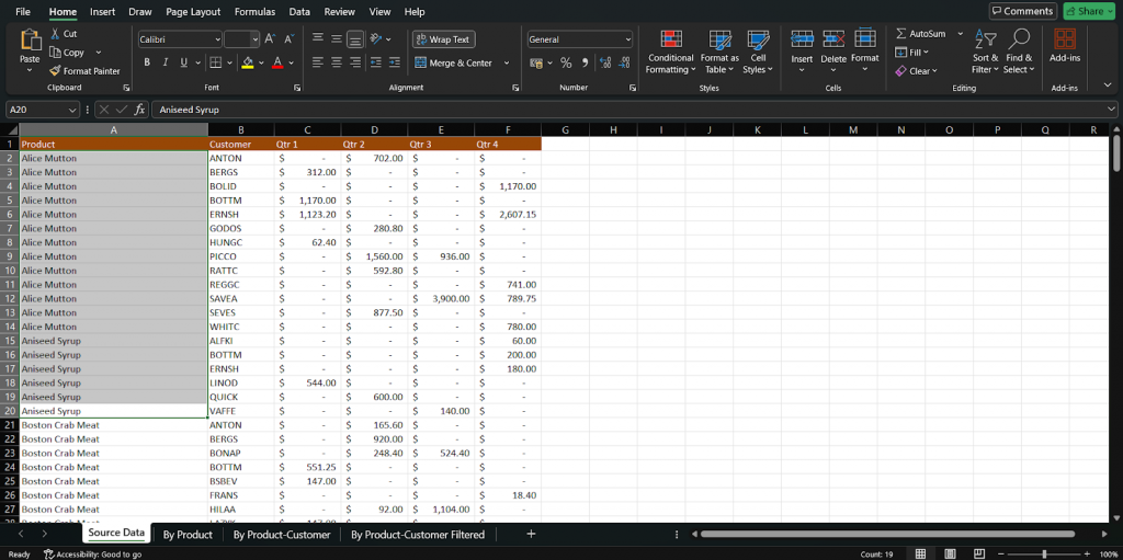
Example: Select cells A2:A20 in case you are highlighting sales figures.
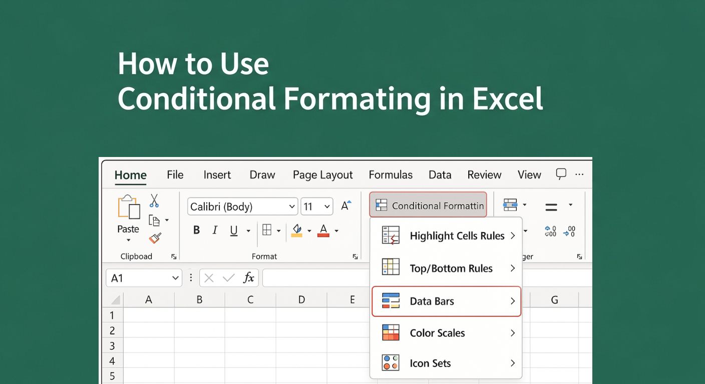
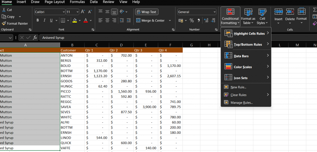
Step 2: Go to Home > Conditional Formatting
Navigate to the Home tab on the Excel ribbon.
In the Styles group, click on Conditional Formatting.
You'll see a drop-down menu with several options like:
- Highlight Cells Rules
- Top/Bottom Rules
- Data Bars
- Color Scales
- Icon Sets
Step 3: Choose a Formatting Rule
From the dropdown, choose the type of rule you want to apply.
Highlight Cell Rules
Apply it to bring out values more than, less than, equal to or between two distinct numbers. It is also possible to highlight cells with some text or dates.
Example: Highlight all values greater than 500 in green.
Top/Bottom Rules
Highlight the top 10 items, bottom 10%, or above-average values.
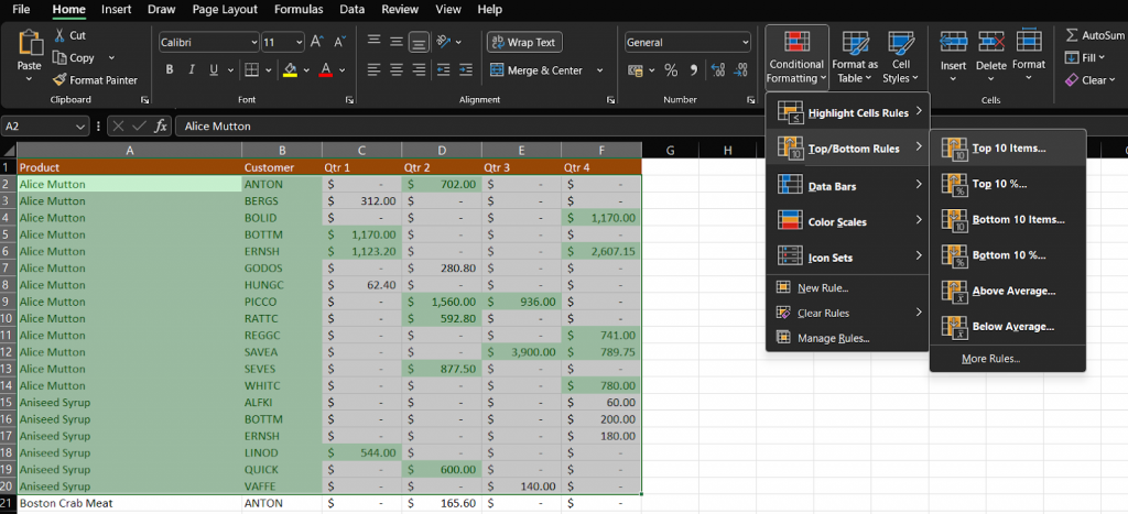
Useful for quick rankings or performance metrics.
Data Bars, Color Scales, Icon Sets
These options create visual cues like horizontal bars, gradient colors, or traffic light icons.
Excellent for doing Visual analysis across Big data.
Step 4: Customize the Formatting
Once you select a rule type, a dialog box will appear.
- Set your criteria (e.g., greater than 500).
- Choose your formatting style (color fill, bold text, etc.).
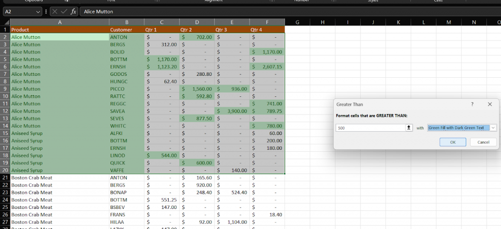
- You can also click Custom Format for more control, like changing font style or adding borders.
Step 5: Click OK
Then, you should click on OK to confirm the rule.
The cells you have selected will now have the conditional formatting according to the rules you have set.
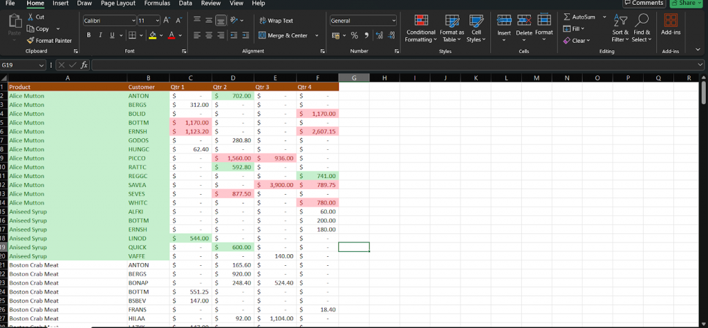
You can add multiple rules to the same range or manage them later via Home > Conditional Formatting > Manage Rules.
Learn Excel for powerful data analysis and enhance your skills for better decision-making.
Pro Tip:
Try combining conditional formatting with Excel formulas (like =AND() or =ISBLANK()) for advanced scenarios. We’ll explore this in a later section.
Use ChatGPT to generate custom Excel formulas faster. Check out this free course on ChatGPT for Excel.
Types of Conditional Formatting Rules in Excel
| Type | Description | Example / Use Case |
| Highlight Cell Rules | Format cells based on values, text, or dates. Options include greater than, less than, between, contains text, or duplicate values. | Highlight sales greater than 1000 in green. |
| Top/Bottom Rules | Emphasize the top 10 items, bottom 10%, or values above/below average. | Identify top-performing employees or underperforming products. |
| Data Bars | Display horizontal bars within cells that visually represent the value in proportion to others in the range. | Track budget utilization or performance scores at a glance. |
| Color Scales | Apply gradient fill colors across a value range, typically from red (low) to green (high), with yellow as a midpoint. | Create heat maps to analyze trends in large datasets. |
| Icon Sets | Use symbols like arrows, flags, or checkmarks to indicate relative values or thresholds. | Build dashboards or visual scorecards with intuitive indicators. |
| Custom Formula-Based Rules | Create custom logic using Excel formulas to determine when formatting should be applied. | =A2>AVERAGE($A$2:$A$20) to highlight above-average sales. Ideal for advanced or dynamic conditions. |
Examples of Conditional Formatting in Action
To better understand how conditional formatting improves data visibility, here are real-world examples of its use:
Example 1: Highlighting Overdue Tasks in a To-Do List
Let’s say you manage a task list with due dates. You can highlight any task past its due date using a formula-based rule:
Formula: =TODAY()>B2 (Assuming B2 contains the due date)
Format: Fill with red
This helps you instantly see what’s overdue without manually checking dates.
Example 2: Color Scale for Sales Data
In a sales report, apply a color scale to a column of monthly revenue. Excel will automatically shade low revenue in red and high revenue in green, with a gradient in between.
This makes it easy to spot trends or regions underperforming.
Example 3: Data Bars to Show Performance Metrics
If you’re tracking employee performance scores out of 100, applying data bars gives a quick, visual comparison:
- Longer bars = higher performance
- Shorter bars = areas for improvement
No need to scan every number, your eyes can interpret the data instantly.
How do I use a Formula in Conditional Formatting?
You can use formulas in conditional formatting to create custom logic beyond the built-in rule types. This is especially useful when you want to format entire rows or apply rules based on multiple conditions.
Common Functions Used in Formula-Based Formatting:
- =AND() – Combines multiple logical conditions.
- =ISBLANK() – Checks if a cell is empty.
- =MOD() – Useful for alternating row colors (e.g., zebra striping).
Formula-based rules allow you to create dynamic formatting tied directly to your logic, making your sheets smarter and more tailored to your needs.
Common Issues and How to Fix Them
1. Formatting Not Applying
- Fix: Double-check the rule logic or formula. Ensure the data type (text vs. number) matches your condition.
2. Wrong Cell References
- Fix: Use absolute ($A$1) or relative (A1) references correctly. Relative references like $C2="Pending" allow formatting to adjust row-by-row.
3. Conflicts Between Rules
- Fix: Go to Home > Conditional Formatting > Manage Rules, check rule priority, and remove or reorder conflicting ones.
Addressing these issues ensures your formatting behaves exactly as intended and improves overall spreadsheet clarity.
Conclusion + Final Tips
Make your data speak with the help of conditional formatting in Excel. Whether you are featuring key values, data visualisations, or problem identification, it aids in the process of making numbers valuable.
It is necessary to start with built-in rules and then venture into custom formulas when you are more confident.
To strengthen your overall Excel skills including formulas, functions, and analytical techniques that enhance formatting and What-If analysis consider enrolling in this Free Excel course for beginners.
Start simple with built-in rules, then explore custom formulas as you grow more confident. Looking to expand your Excel skills? Check out our related tutorials on:
- How to Use VLOOKUP in Excel
- Top Excel Formulas List
- How to Create Pivot Tables in Excel
- Excel Quiz to Test Your Knowledge
Frequently Asked Questions (FAQs)
Q1: Can I use conditional formatting across multiple sheets in Excel?
A: No, conditional formatting rules apply only to the sheet where they’re created. In case of similar formatting in other sheet, you will have to manually redo or copy the formatting.
Q2: Will conditional formatting slow down Excel?
A: In most cases, no. But when you use formula-based rules on thousands of cells particularly in large sheets, then it might affect the performance slightly. Use effective formulas and make formatting within the minimum ranges possible.
Q3: How do I remove conditional formatting?
A: Select Home > Conditional Formatting > Clear Rules, after which one may decide to clear the formatting in the selected cells, or clear the whole sheet. You can also delete or manage particular rules through Manage Rules..
Q4: Can I copy conditional formatting to another range?A: Yes! The same format rules can be applied to another range using Format Painter. All you need is to single-click the cell that has the format, choose Format Painter, and highlight the new range.