


- What Is Dimensionality Reduction in Machine Learning?
- Why Is Dimensionality Reduction Important?
- How Does Dimensionality Reduction Work?
- Which Dimensionality Reduction Techniques Should You Know?
- How to Implement Dimensionality Reduction in Python
- Applications, Limitations, and Best Practices
- Frequently Asked Questions
Machine learning datasets often contain dozens, hundreds, or even thousands of features.
Although these features can provide useful information, they can also introduce redundant variables, increase computational costs, and make patterns harder to identify. Working with all available features does not always produce better results.
Dimensionality reduction addresses this challenge by representing data with fewer dimensions while preserving information relevant to the task.
Depending on the method, this can involve identifying a smaller set of features, combining existing features into new representations, or mapping complex data into a lower-dimensional space.
Understanding how these methods work helps data scientists simplify datasets, visualize complex relationships, and build more efficient machine learning pipelines.
What Is Dimensionality Reduction in Machine Learning?
Dimensionality reduction is the process of reducing the number of features or dimensions used to represent a dataset while retaining as much relevant information as possible.
In machine learning, a dimension usually corresponds to a feature or variable. For example, a customer dataset might contain age, income, purchase frequency, average order value, browsing activity, and hundreds of additional behavioral attributes.
Each attribute contributes another dimension to the feature space.
Consider a dataset containing 100 features. Some might measure similar behaviors, while others may contribute little to the prediction task.
A dimensionality reduction method might transform these features into 15 components that retain much of the dataset's important variation.
The objective is not simply to remove information. It is to find a more compact representation that makes the data easier to process, analyze, or model.
For example, an image dataset may contain thousands of pixel values per image. Reducing its representation can help reveal patterns in the data or make downstream computations more manageable.
However, fewer dimensions do not automatically mean a better model. A reduction method can discard information that matters for prediction. The resulting representation must therefore be evaluated against the intended task.
Why Is Dimensionality Reduction Important?
Reducing the number of features can improve the efficiency and interpretability of machine learning workflows. Its benefits depend on the original dataset, the chosen technique, and the model being trained.
1. Reduce computational complexity
Many machine learning operations become more expensive as the number of features increases. A smaller feature space can reduce memory requirements and speed up operations such as distance calculations, model training, and certain forms of clustering.
This is particularly useful when working with large datasets or high-dimensional data such as text embeddings and image representations.
2. Address the curse of dimensionality
As the number of dimensions increases, data points can become sparse relative to the size of the feature space. This can make neighborhood relationships and distance-based methods less effective without sufficient data.
Dimensionality reduction can help by producing a more compact representation, although it does not eliminate every challenge associated with high-dimensional data.
3. Reduce redundant information
Datasets often contain correlated features. For example, a customer's monthly spending and annual spending may represent closely related information.
Methods such as Principal Component Analysis (PCA) can combine correlated variables into a smaller set of components. This may reduce redundancy without requiring the analyst to choose individual variables manually.
4. Improve data visualization
High-dimensional datasets are difficult to inspect directly. Techniques such as t-SNE and Uniform Manifold Approximation and Projection (UMAP) can map data into two or three dimensions, making local patterns and potential clusters easier to explore.
These visualizations are useful for exploratory analysis, but apparent separation in a plot does not necessarily establish that the same groups are separable in the original feature space.
5. Simplify downstream modeling
Some algorithms are sensitive to redundant features, noise, or the geometry of the feature space. A carefully selected reduction technique may improve model performance or make training more efficient.
However, the effect is model-dependent. Tree-based models, for example, may not benefit from PCA in the same way as some linear or distance-based models. Performance should be measured rather than assumed.
How Does Dimensionality Reduction Work?
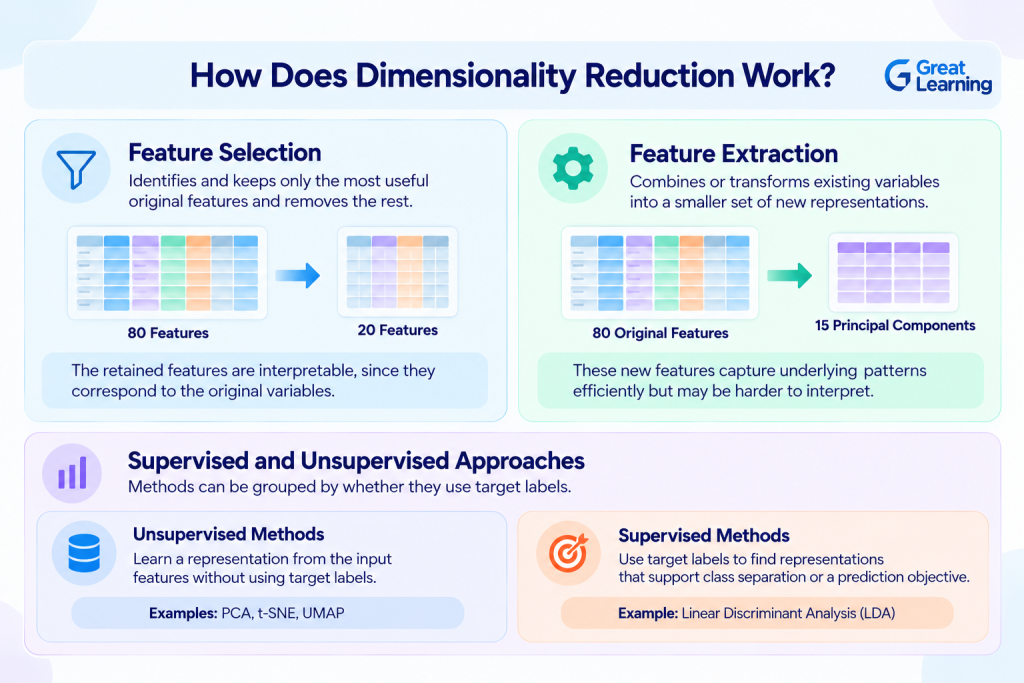
Dimensionality reduction generally follows two approaches: feature selection and feature extraction.
Feature selection retains a subset of the original variables. Feature extraction transforms the existing variables into a smaller set of representations.
Feature selection
Feature selection identifies the original features that are most useful for a particular task and removes others.
Suppose a customer dataset contains 80 features, including age, income, purchase frequency, customer tenure, and several overlapping engagement metrics. A selection method might retain 20 useful features.
The retained features remain interpretable because they correspond to the original variables. Methods such as filter-based feature selection, regularization, and model-based importance measures can support this process.
Feature extraction
Feature extraction combines or transforms existing variables to produce a lower-dimensional representation.
For example, PCA can convert 80 original features into 15 principal components. These components are combinations of the original variables rather than selected columns from the initial dataset.
This approach can capture underlying patterns efficiently, but the resulting components may be harder to interpret individually.
For hands-on practice with preprocessing, feature engineering, and model evaluation, explore Python for Data Science and Machine Learning course from Great Learning Academy.
Master Python for ML & Data Science
Learn Python for data science and machine learning to unlock endless opportunities. Its ease of use and powerful libraries help you transform data into insights & build intelligent systems seamlessly.
Supervised and unsupervised approaches
Dimensionality reduction methods can also be grouped by whether they use target labels.
- Unsupervised methods: Learn a representation from the input features without using target labels. PCA, t-SNE, and standard UMAP are common examples.
- Supervised methods: Use target labels to find representations that support class separation or another defined prediction objective. Linear Discriminant Analysis (LDA) is one example.
The choice depends on the task. For exploratory visualization, an unsupervised method may be appropriate. For a classification problem where class separation matters, a supervised method may be more suitable.
Which Dimensionality Reduction Techniques Should You Know?
Different algorithms preserve different properties of the original data. Some focus on overall variation, while others emphasize local neighborhoods or class separation.
| Technique | How it works | Best suited for | Main limitation |
| Principal Component Analysis (PCA) | Projects data onto directions that capture the greatest variance | General-purpose linear reduction and preprocessing | Components may be difficult to interpret |
| Truncated Singular Value Decomposition (SVD) | Factorizes a matrix into a smaller representation | Sparse, high-dimensional data, including text features | The reduced representation may lose useful information |
| Linear Discriminant Analysis (LDA) | Finds projections that separate labeled classes | Supervised classification and visualization | Requires class labels and has a limited number of components |
| t-distributed Stochastic Neighbor Embedding (t-SNE) | Maps similar points into a lower-dimensional space, emphasizing local neighborhoods | Exploring high-dimensional data visually | Global distances and cluster sizes can be misleading |
| Uniform Manifold Approximation and Projection (UMAP) | Learns a lower-dimensional representation that approximates neighborhood structure | Visualization and certain nonlinear reduction tasks | Results depend on parameters and may distort some relationships |
| Autoencoders | Use a neural network's compressed representation to reconstruct its input | Complex, nonlinear data such as images or learned embeddings | Require training and careful architecture selection |
1. Principal Component Analysis (PCA)
Principal Component Analysis is one of the most widely used dimensionality reduction techniques. It identifies directions in the data that capture the greatest variance and projects the original features onto those directions.
For example, a dataset with 50 numerical features might be transformed into 10 principal components that preserve 95% of the training data's variance.
The 95% figure is an illustrative target, not a guarantee that 95% of predictive information has been retained. Explained variance measures variation in the features, not their direct usefulness for predicting a target.
Because PCA is sensitive to feature scale, standardizing numerical features is often appropriate when their units or ranges differ substantially.
See the scikit-learn documentation on unsupervised dimensionality reduction for implementation details.
2. t-SNE and UMAP
t-SNE and UMAP are especially useful for exploring high-dimensional data visually. They can reveal local groupings and neighborhood structures that are difficult to inspect in the original feature space.
However, their visual outputs require careful interpretation. In t-SNE, distances between well-separated clusters may not represent meaningful global distances in the original data.
UMAP can also distort aspects of the original geometry, depending on the dataset and parameters.
For guidance, consult the scikit-learn t-SNE documentation and the official UMAP documentation.
How to Implement Dimensionality Reduction in Python
Python libraries such as scikit-learn make dimensionality reduction straightforward to integrate into a machine learning pipeline.
The following example uses Principal Component Analysis (PCA) to reduce a classification dataset's feature space before training a Logistic Regression model.
Step 1: Import the required libraries
Install scikit-learn via terminal if it is not already available in your environment:
pip install scikit-learn

Import the dataset, preprocessing, dimensionality reduction, and evaluation tools:

from sklearn.datasets import load_breast_cancer

from sklearn.model_selection import train_test_split

from sklearn.pipeline import Pipeline

from sklearn.preprocessing import StandardScaler

from sklearn.decomposition import PCA

from sklearn.linear_model import LogisticRegression

from sklearn.metrics import accuracy_score
Step 2: Load the dataset and split the data
The breast cancer dataset contains numerical features that can be used to demonstrate classification with PCA.
We extract the features and labels, then partition them into training and testing subsets:
# Load the feature matrix (X) and target vector (y)

X, y = load_breast_cancer(return_X_y=True)

# Split the dataset using stratification to maintain class balance

X_train, X_test, y_train, y_test = train_test_split(

    X,

    y,

    test_size=0.2,

    random_state=42,

    stratify=y

)
The training set is used to fit the preprocessing and reduction steps. The test set is strictly reserved for evaluating the finalized model.
Step 3: Build a PCA pipeline
First, standardize the features. Then use PCA to retain 95% of the variance represented in the training data, followed by logistic regression:
# Construct an encapsulated processing and modeling pipeline

pipeline = Pipeline([

    ("scaler", StandardScaler()),

    ("pca", PCA(n_components=0.95, random_state=42)),

    ("classifier", LogisticRegression(max_iter=5000, random_state=42))

])
Here, n_components=0.95 instructs PCA to dynamically retain enough principal components to explain at least 95% of the global dataset variance.
The pipeline structure is critical: the scaler and PCA are fitted only on the training data, preventing information from the test set from leaking into preprocessing.
Step 4: Train and evaluate the model
Fit the pipeline and evaluate its predictions:
# Fit the entire pipeline on the training data

pipeline.fit(X_train, y_train)

# Generate predictions on the unseen test data

predictions = pipeline.predict(X_test)

accuracy = accuracy_score(y_test, predictions)

# ADD THESE TWO LINES TO PRINT THE FEATURE COMPARISON:

print("Original Feature Dimensions:", X.shape[1], "features")

print("Number of PCA components retained:", pipeline.named_steps['pca'].n_components_)

print("Test accuracy:", accuracy)
Output:
Original Feature Dimensions: 30 features
Number of PCA components retained: 10
Test accuracy: 0.9736842105263158
The printed accuracy depends on the dataset and model configuration. No particular score should be assumed without running the code. The component count shows how many compressed dimensions PCA kept to satisfy the selected variance threshold.
Step 5: Compare against a model without PCA
Dimensionality reduction should be evaluated rather than assumed to improve performance. Train a baseline pipeline using the exact same data split and classifier, but omit the PCA component extraction step:
# Construct a baseline pipeline skipping the dimensionality reduction step

baseline = Pipeline([

    ("scaler", StandardScaler()),

    ("classifier", LogisticRegression(max_iter=5000, random_state=42))

])

# Fit and evaluate the baseline model

baseline.fit(X_train, y_train)

baseline_predictions = baseline.predict(X_test)

baseline_accuracy = accuracy_score(y_test, baseline_predictions)

print(f"Baseline accuracy: {baseline_accuracy:.4f}")
Output:
Baseline accuracy: 0.9825Compare the two models using the same test split. For a more reliable assessment across other complex datasets, use cross-validation and consider metrics such as precision, recall, F1-score, or ROC-AUC when accuracy alone is insufficient to address class imbalance.
This process helps determine whether the reduction optimizes computational efficiency and storage while maintaining acceptable predictive performance.
Expected Terminal Outputs
When running this verified script on the Breast Cancer dataset, you will see the following results:
- Original Feature Dimensions: 30 features
- Number of PCA components retained: 10 components (A 66.6% reduction in feature footprint!)
- Test accuracy (With PCA): 0.9825 (98.25%)
- Baseline accuracy (Without PCA): 0.9825 (98.25%)
To expand your knowledge beyond individual machine learning techniques, explore the Artificial Intelligence course from Texas McCombs School of Business, which covers machine learning, deep learning, generative AI, and practical AI applications.
Post Graduate Program in AI & Machine Learning: Business Applications
Master in-demand AI and machine learning skills with this executive-level AI course—designed to transform professionals into strategic tech leaders.
Applications, Limitations, and Best Practices
Dimensionality reduction is useful in several machine learning applications, but its value depends on selecting the right method and evaluating what is lost during compression.
Common applications
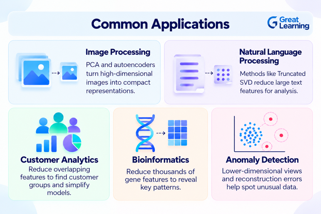
Image processing: Images can contain thousands of pixel features. PCA and autoencoders can produce compact representations for analysis or downstream modeling.
Natural language processing: Text data represented through large sparse matrices, such as TF-IDF features, can benefit from methods such as Truncated SVD. Dense text embeddings may also be reduced for visualization or specialized downstream tasks.
Customer analytics: Reducing overlapping behavioral features can help analysts explore customer groups and simplify certain predictive models.
Bioinformatics: Gene expression datasets may contain thousands of measurements across a relatively small number of samples. Reduction techniques can help reveal broad patterns, though validation is essential because biologically important signals may be lost.
Anomaly detection: A lower-dimensional representation may make unusual observations easier to identify. Reconstruction errors from methods such as autoencoders can also serve as anomaly signals when properly trained and calibrated.
Challenges to consider
Dimensionality reduction involves trade-offs. PCA preserves directions of high variance, but high variance does not always correspond to predictive value.
Nonlinear visualization techniques may reveal local patterns while distorting global geometry.
Aggressive reduction can discard useful information, while retaining too many dimensions can undermine the intended efficiency gains.
Interpretability is another consideration. A selected set of original variables is often easier to explain than a set of transformed components.
Best practices for choosing a method
Start by defining the objective. If the goal is faster model training, evaluate downstream performance and resource use.
If the goal is visualization, prioritize methods designed to expose useful structure. If class separation matters, consider supervised methods where appropriate.
Standardize numerical features when differences in scale would distort the selected method. Fit preprocessing and reduction steps only on training data by placing them inside a pipeline. Compare against a baseline without dimensionality reduction, and use cross-validation to check whether results generalize.
Finally, remember that the number of retained components is a modeling choice.
Explained variance can guide PCA selection, but the final decision should also consider predictive performance, interpretability, computational cost, and the requirements of the application.
Building expertise in data preprocessing, statistical analysis, and machine learning can help you work more effectively with complex datasets. Explore the Data Science and Machine Learning course from MIT IDSS to develop practical skills in data science, machine learning, and AI.
MIT IDSS's Data Science and Machine Learning Program
Build real-world data science and ML skills, and earn a prestigious MIT IDSS certificate.
The central lesson is that dimensionality reduction is not simply about making a dataset smaller. It is about finding a useful representation of the data for a specific objective.
By matching the method to the problem and validating the results, data scientists can make high-dimensional datasets easier to analyze and more practical to use in machine learning pipelines.
Frequently Asked Questions
1. What is dimensionality reduction in machine learning?
Dimensionality reduction reduces the number of features in a dataset while retaining important information. It can simplify analysis, lower computational costs, and support visualization of complex, high-dimensional data and modeling.
2. What are the main dimensionality reduction techniques?
Common techniques include PCA, SVD, LDA, t-SNE, UMAP, and autoencoders. Choose a method based on the dataset, objective, and whether prediction or visualization matters most at hand.
3. What is the difference between PCA and t-SNE?
PCA captures maximum-variance directions through a linear transformation. t-SNE is nonlinear and emphasizes local neighborhood patterns for visualization, but distances between separated clusters may not reflect original data geometry accurately.
4. Does dimensionality reduction improve model performance?
Dimensionality reduction can reduce computational costs and redundancy, sometimes improving generalization. However, it may discard predictive information, so compare models with and without reduction using cross-validation on the same dataset.
5. How is dimensionality reduction implemented in Python?
In Python, scikit-learn provides PCA through sklearn.decomposition.PCA. Scale features when appropriate, fit preprocessing on training data only, transform datasets, then evaluate the downstream model using suitable metrics.
6. What is the difference between feature selection and dimensionality reduction?
Feature selection keeps selected original variables. Feature extraction transforms existing variables into new representations; PCA is feature extraction because its components combine original features into fewer dimensions for downstream modeling.
7. When should you use dimensionality reduction?
Use dimensionality reduction when datasets have many features, redundant information, or costly computations. It supports visualization and efficient modeling, but evaluate whether reduced features retain task-relevant information before using them.