- What is Feature Extraction?
- Why Feature Extraction is Useful?
- Applications of Feature Extraction
- How to Store Images in the Machine?
- How to use Feature Extraction technique for Image Data: Features as Grayscale Pixel Value
- How to extract features from Image Data: What is the Mean pixel value in channel?
- Project Using Feature Extraction technique
- Background of OpenCV:
- Image feature Detection using OpenCV:
- Further Reading
In real life, all the data we collect are in large amounts. To understand this data, we need a process. Manually, it is not possible to process them. Here's when the concept of feature extraction comes in.
Suppose you want to work with some of the big machine learning projects or the coolest and most popular domains such as deep learning, where you can use images to make a project on object detection. Making projects on computer vision where you can work with thousands of interesting projects in the image data set. To work with them, you have to go for feature extraction, take up a digital image processing course and learn image processing in Python which will make your life easy. Upskilling with the help of a free online course will help you understand the concepts clearly.
So let's have a look at how we can use this technique in a real scenario.
- What is feature extraction?
- Why Feature extraction is useful?
- Applications of feature extraction
- How to Store Images in the Machine?
- How to use Feature Extraction technique for Image Data: Features as Grayscale Pixel Values
- How to extract features from Image Data: What is the Mean Pixel Value of Channels
- Project Using Feature Extraction technique
- Image feature detection using OpenCV
What is Feature Extraction?
Feature extraction is a part of the dimensionality reduction process, in which, an initial set of the raw data is divided and reduced to more manageable groups. So when you want to process it will be easier. The most important characteristic of these large data sets is that they have a large number of variables. These variables require a lot of computing resources to process. So Feature extraction helps to get the best feature from those big data sets by selecting and combining variables into features, thus, effectively reducing the amount of data. These features are easy to process, but still able to describe the actual data set with accuracy and originality.
Why Feature Extraction is Useful?
The technique of extracting the features is useful when you have a large data set and need to reduce the number of resources without losing any important or relevant information. Feature extraction helps to reduce the amount of redundant data from the data set.
In the end, the reduction of the data helps to build the model with less machine effort and also increases the speed of learning and generalization steps in the machine learning process.
Master AI with Microsoft AI Professional Program
Gain industry-ready AI skills through real-world projects and earn a Microsoft-recognized certification to elevate your tech career.
Applications of Feature Extraction
- Bag of Words- Bag-of-Words is the most used technique for natural language processing. In this process they extract the words or the features from a sentence, document, website, etc. and then they classify them into the frequency of use. So in this whole process feature extraction is one of the most important parts.
- Image Processing –Image processing is one of the best and most interesting domain. In this domain basically you will start playing with your images in order to understand them. So here we use many many techniques which includes feature extraction as well and algorithms to detect features such as shaped, edges, or motion in a digital image or video to process them.
- Auto-encoders: The main purpose of the auto-encoders is efficient data coding which is unsupervised in nature. this process comes under unsupervised learning . So Feature extraction procedure is applicable here to identify the key features from the data to code by learning from the coding of the original data set to derive new ones.
How to Store Images in the Machine?
So in this section, we will start from scratch. For the first thing, we need to understand how a machine can read and store images. Loading the image, reading them, and then process them through the machine is difficult because the machine does not have eyes like us.
Let's have a look at how a machine understands an image.
Machines see any images in the form of a matrix of numbers. The size of this matrix actually depends on the number of pixels of the input image.
What is a pixel?
The Pixel Values for each of the pixels stands for or describes how bright that pixel is, and what color it should be. So In the simplest case of the binary images, the pixel value is a 1-bit number indicating either foreground or background.
So pixels are the numbers or the pixel values which denote the intensity or brightness of the pixel.
Smaller numbers that are closer to zero helps to represent black, and the larger numbers which are closer to 255 denote white.
So this is the concept of pixels and how the machine sees the images without eyes through the numbers.

The dimensions of the image are 28 x 28. And if you want to check then by counting the number of pixels you can verify.
But, for the case of a colored image, we have three Matrices or the channels
- Red,
- Green
- and Blue.
So in these three matrices, each of the matrix has values between 0-255 which represents the intensity of the color of that pixel.
If you have a colored image like the dog image we have in the above image on the left. so being a human you have eyes so you can see and can say it is a dog-colored image. But how a computer can understand it is the colored or black and white image?
So you can see we also have three matrices that represent the channel of RGB - (for the three color channels – Red, Green, and Blue) On the right, we have three matrices. These three channels are superimposed and used to form a colored image. So this is how a computer can differentiate between the images.
Let's have an example of how we can execute the code using Python
import pandas as pd
import numpy as np
import matplotlib.pyplot as plt
%matplotlib inline

from skimage.io import imread, imshow
image = imread('/content/sample_image.png', as_gray=True)
imshow(image)

Check the shape of the image:
#check the image shape
print(image.shape)

print(image)
Image shape: (1480, 1490)
Array:
[[0.96862745 0.96862745 0.79215686 ... 0.96862745 1. 1. ] [0.96862745 0.96862745 0.79215686 ... 0.96862745 1. 1. ] [0.79215686 0.79215686 0. ... 0.79215686 1. 1. ] ... [0.89019608 0.89019608 0. ... 0.89019608 1. 1. ] [0.8745098 0.8745098 0. ... 0.8745098 1. 1. ] [0.8745098 0.8745098 0. ... 0.8745098 1. 1. ]]
How to use Feature Extraction technique for Image Data: Features as Grayscale Pixel Value
If we use the same example as our image which we use above in the section– the dimension of the image is 28 x 28 right? But can you guess the number of features for this image?
The number of features is same as the number of pixels so that the number will be 784
So now I have one more important question –
how do we declare these 784 pixels as features of this image? Do you ever think about that?
So the solution is, you just can simply append every pixel value one after the other to generate a feature vector for the image. Let's visualize that,

Now let's have a look at the coloured image,
image = imread('/content/pexels-photo-1108099.jpeg')
imshow(image)

print(image.shape)
(375, 500, 3)
image
array([[[ 74, 95, 56], [ 74, 95, 56], [ 75, 96, 57], ..., [ 73, 93, 56], [ 73, 93, 56], [ 72, 92, 55]], [[ 74, 95, 56], [ 74, 95, 56], [ 75, 96, 57], ..., [ 73, 93, 56], [ 73, 93, 56], [ 72, 92, 55]], [[ 74, 95, 56], [ 75, 96, 57], [ 75, 96, 57], ..., [ 73, 93, 56], [ 73, 93, 56], [ 73, 93, 56]], ..., [[ 71, 85, 50], [ 72, 83, 49], [ 70, 80, 46], ..., [106, 93, 51], [108, 95, 53], [110, 97, 55]], [[ 72, 86, 51], [ 72, 83, 49], [ 71, 81, 47], ..., [109, 90, 47], [113, 94, 51], [116, 97, 54]], [[ 73, 87, 52], [ 73, 84, 50], [ 72, 82, 48], ..., [113, 89, 45], [117, 93, 49], [121, 97, 53]]], dtype=uint8)
image = imread('/content/pexels-photo-1108099.jpeg', as_gray=True)
image.shape, imshow(image)

print(image.shape)
(375, 500)
image
array([[0.34402196, 0.34402196, 0.34794353, ..., 0.33757765, 0.33757765, 0.33365608], [0.34402196, 0.34402196, 0.34794353, ..., 0.33757765, 0.33757765, 0.33365608], [0.34402196, 0.34794353, 0.34794353, ..., 0.33757765, 0.33757765, 0.33757765], ..., [0.31177059, 0.3067102 , 0.29577882, ..., 0.36366392, 0.37150706, 0.3793502 ], [0.31569216, 0.3067102 , 0.29970039, ..., 0.35661647, 0.37230275, 0.38406745], [0.31961373, 0.31063176, 0.30362196, ..., 0.35657882, 0.3722651 , 0.38795137]])
The image shape for this image is 375 x 500. So, the number of features will be 187500.
o now if you want to change the shape of the image that is also can be done by using the reshape function from NumPy where we specify the dimension of the image:
#Find the pixel features
feature = np.reshape(image, (375*500))
feature.shape
(187500,)
features
array([0.34402196, 0.34402196, 0.34794353, ..., 0.35657882, 0.3722651 , 0.38795137])
PG Program in AI & Machine Learning
Master AI with hands-on projects, expert mentorship, and a prestigious certificate from UT Austin and Great Lakes Executive Learning.
How to extract features from Image Data: What is the Mean pixel value in channel?
So here we will start with reading our coloured image. Here we did not us the parameter "as_gray = True’
image = imread('/content/pexels-photo-1108099.jpeg')
imshow(image)
print(image.shape)
(375, 500, 3)
image
array([[[ 74, 95, 56], [ 74, 95, 56], [ 75, 96, 57], ..., [ 73, 93, 56], [ 73, 93, 56], [ 72, 92, 55]], [[ 74, 95, 56], [ 74, 95, 56], [ 75, 96, 57], ..., [ 73, 93, 56], [ 73, 93, 56], [ 72, 92, 55]], [[ 74, 95, 56], [ 75, 96, 57], [ 75, 96, 57], ..., [ 73, 93, 56], [ 73, 93, 56], [ 73, 93, 56]], ..., [[ 71, 85, 50], [ 72, 83, 49], [ 70, 80, 46], ..., [106, 93, 51], [108, 95, 53], [110, 97, 55]], [[ 72, 86, 51], [ 72, 83, 49], [ 71, 81, 47], ..., [109, 90, 47], [113, 94, 51], [116, 97, 54]], [[ 73, 87, 52], [ 73, 84, 50], [ 72, 82, 48], ..., [113, 89, 45], [117, 93, 49], [121, 97, 53]]], dtype=uint8)
For this scenario the image has a dimension (375,500,3). This three represents the RGB value as well as the number of channels. Now we will use the previous method to create the features.
The total number of features will be for this case 375*500*3 = 562500

From the past, we are all aware that, the number of features remains the same. In this case, the pixel values from all three channels of the image will be multiplied.
Now we will implement this using Python:
image = imread('/content/pexels-photo-1108099.jpeg')
feature_matrix_image = np.zeros((375,500))
feature_matrix_image
array([[0., 0., 0., ..., 0., 0., 0.], [0., 0., 0., ..., 0., 0., 0.], [0., 0., 0., ..., 0., 0., 0.], ..., [0., 0., 0., ..., 0., 0., 0.], [0., 0., 0., ..., 0., 0., 0.], [0., 0., 0., ..., 0., 0., 0.]])
feature_matrix_image.shape
(375, 500)
In this coloured image has a 3D matrix of dimension (375*500 * 3) where 375 denotes the height, 500 stands for the width and 3 is the number of channels. In order to get the average pixel values for the image, we will use a for loop:
for i in range(0,image.shape[0]):

    for j in range(0,image.shape[1]):

        feature_matrix_image[i][j] = ((int(image[i,j,0]) + int(image[i,j,1]) + int(image[i,j,2]))/3)
feature_matrix_image
array([[75. , 75. , 76. , ..., 74. , 74. , 73. ], [75. , 75. , 76. , ..., 74. , 74. , 73. ], [75. , 76. , 76. , ..., 74. , 74. , 74. ], ..., [68.66666667, 68. , 65.33333333, ..., 83.33333333, 85.33333333, 87.33333333], [69.66666667, 68. , 66.33333333, ..., 82. , 86. , 89. ], [70.66666667, 69. , 67.33333333, ..., 82.33333333, 86.33333333, 90.33333333]])
feature_matrix_image.shape
(375, 500)
Now we will make a new matrix that will have the same height and width but only 1 channel.
To convert the matrix into a 1D array we will use the Numpy library,
feature_sample = np.reshape(feature_matrix_image, (375*500))

feature_sample
array([75. , 75. , 76. , ..., 82.33333333, 86.33333333, 90.33333333])
feature_sample.shape
(187500,)
Project Using Feature Extraction technique
Importing an Image
To import an image we can use Python pre-defined libraries
import pandas as pd

import numpy as np

import matplotlib.pyplot as plt

%matplotlib inline

from skimage.io import imread, imshow

image = imread("/content/pexels-photo-1108099.jpeg")

imshow(image)
Introduction to OpenCV:
There are some predefined packages and libraries are there to make our life simple.
One of the most important and popular libraries is Opencv. It helps us to develop a system that can process images and real-time video using computer vision. OpenCv focused on image processing, real-time video capturing to detect faces and objects.
Background of OpenCV:
OpenCV was invented by Intel in 1999 by Gary Bradsky. The first release was in the year 2000. OpenCV stands for Open Source Computer Vision Library. This Library is based on optimized C/C++ and it supports Java and Python along with C++ through interfaces.
OpenCV is one of the most popular and successful libraries for computer vision and it has an immense number of users because of its simplicity, processing time and high demand in computer vision applications. OpenCV-Python is like a python wrapper around the C++ implementation. OpenCv has more than 2500 implemented algorithms that are freely available for commercial purpose as well.
- Applications of OpenCV:
- Medical image analysis: We all know image processing in the medical industry is very popular.
Let’s take an example:
Identify Brain tumour: Every single day almost thousands of patients are dealing with brain tumours. There are many software which are using OpenCv to detect the stage of the tumour using an image segmentation technique.
One of the applications is RSIP Vision which builds a probability map to localize the tumour and uses deformable models to obtain the tumour boundaries with zero level energy.
- Object Detection: Detecting objects from the images is one of the most popular applications.
Suppose,
You want to detect a person sitting on a two-wheeler vehicle without a helmet which is equivalent to a defensible crime.
So you can make a system that detects the person without a helmet and captures the vehicle number to add a penalty.
There are many applications there using OpenCv which are really helpful and efficient. These applications are also taking us towards a more advanced world with less human effort.
Image feature Detection using OpenCV:
import cv2

import numpy as np

import cv2

import matplotlib.pyplot as plt

%matplotlib inline
img_load = cv2.imread("/content/toppng.com-service-dogs-tv-pg-dog-pictures-white-background-628x669.png")
img_load
array([[[ 76, 112, 71], [ 76, 112, 71], [ 76, 112, 71], ..., [ 76, 112, 71], [ 76, 112, 71], [ 76, 112, 71]], [[ 76, 112, 71], [ 76, 112, 71], [ 76, 112, 71], ..., [ 76, 112, 71], [ 76, 112, 71], [ 76, 112, 71]], [[ 76, 112, 71], [ 76, 112, 71], [ 76, 112, 71], ..., [ 76, 112, 71], [ 76, 112, 71], [ 76, 112, 71]], ..., [[ 76, 112, 71], [ 76, 112, 71], [ 76, 112, 71], ..., [ 21, 31, 41], [ 21, 31, 41], [ 21, 31, 41]], [[ 76, 112, 71], [ 76, 112, 71], [ 76, 112, 71], ..., [114, 168, 219], [ 21, 31, 41], [ 76, 112, 71]], [[ 76, 112, 71], [ 76, 112, 71], [ 76, 112, 71], ..., [110, 167, 221], [106, 155, 203], [ 76, 112, 71]]], dtype=uint8)
from google.colab.patches import cv2_imshow

cv2_imshow(img_load)

img_load1 = cv2.cvtColor(img_load, cv2.COLOR_BGR2RGB)  # Convert from cv's BRG default color order to RGB
img_load1
array([[[ 71, 112, 76], [ 71, 112, 76], [ 71, 112, 76], ..., [ 71, 112, 76], [ 71, 112, 76], [ 71, 112, 76]], [[ 71, 112, 76], [ 71, 112, 76], [ 71, 112, 76], ..., [ 71, 112, 76], [ 71, 112, 76], [ 71, 112, 76]], [[ 71, 112, 76], [ 71, 112, 76], [ 71, 112, 76], ..., [ 71, 112, 76], [ 71, 112, 76], [ 71, 112, 76]], ..., [[ 71, 112, 76], [ 71, 112, 76], [ 71, 112, 76], ..., [ 41, 31, 21], [ 41, 31, 21], [ 41, 31, 21]], [[ 71, 112, 76], [ 71, 112, 76], [ 71, 112, 76], ..., [219, 168, 114], [ 41, 31, 21], [ 71, 112, 76]], [[ 71, 112, 76], [ 71, 112, 76], [ 71, 112, 76], ..., [221, 167, 110], [203, 155, 106], [ 71, 112, 76]]], dtype=uint8)
cv2_imshow(img_load1)

#converting image to Gray scale

gray_image = cv2.cvtColor(img_load,cv2.COLOR_BGR2GRAY)

#plotting the grayscale image

cv2_imshow(gray_image)

#converting image to HSV format

hsv_image_load = cv2.cvtColor(img_load,cv2.COLOR_BGR2HSV)

#plotting the HSV image

cv2_imshow(hsv_image_load)

#converting image to size (100,100,3)

smaller_image_size = cv2.resize(img_load,(100,100))
cv2_imshow(smaller_image_size)

rows,colums = img_load.shape[:2]

#(col/2,rows/2) is the center of rotation for the image

# M is the cordinates of the center

M_load = cv2.getRotationMatrix2D((colums/2,rows/2),90,1)

dst_load = cv2.warpAffine(img_load,M_load,(cols,rows))

cv2_imshow(dst_load)

ret,thresh_binary = cv2.threshold(gray_image,127,255,cv2.THRESH_BINARY)

ret,thresh_binary_inv = cv2.threshold(gray_image,127,255,cv2.THRESH_BINARY_INV)

ret,thresh_trunc = cv2.threshold(gray_image,127,255,cv2.THRESH_TRUNC)

ret,thresh_tozero = cv2.threshold(gray_image,127,255,cv2.THRESH_TOZERO)

ret,thresh_tozero_inv = cv2.threshold(gray_image,127,255,cv2.THRESH_TOZERO_INV)
#DISPLAYING THE DIFFERENT THRESHOLDING STYLES using OpenCV

names = ['Oiriginal Image','BINARY','THRESH_BINARY','THRESH_TRUNC','THRESH_TOZERO','THRESH_TOZERO_INV']

images = gray_image,thresh_binary,thresh_binary_inv,thresh_trunc,thresh_tozero,thresh_tozero_inv

for i in range(6):

    plt.subplot(2,3,i+1),plt.imshow(images[i],'gray')

    plt.title(names[i])

    plt.xticks([]),plt.yticks([])

Edge detection:
#calculate the edges using Canny edge algorithm

edges_of_image = cv2.Canny(img_load,100,200)

#plot the edges

cv2_imshow(edges_of_image)

This brings us to the end of this article where we learned about feature extraction.