Browse by Domains

What is Recurrent Neural Network | Introduction of Recurrent Neural Network

Before starting with neural networks, let’s have a look at the basics of neural networks.

Neural networks are considered as the most powerful and widely used algorithms. It is the subfield of machine learning which is called deep learning. For the beginners who just start their journey with neural networks, for them maybe neural networks seem like a black box.

So let me give you a small idea how the magic happens, so the neural network has an input layer which receives the input data and then those data goes into the “hidden layers” and after a magic trick, those information comes to the output layer

So what is that magic and magic tricks? 

Now we will understand about those magic tricks which are called hidden layers in the neural network.

What is a Neural network?

The neural networks come under the subfield of artificial neural networks.

But what is Artificial Intelligence?

As the name suggests, Artificial Intelligence is based on the Human brain technique.

This is implemented based on what science knows about the human brain’s structure and function and how it works.

In short Neural network stands as a computing system which consists of highly interconnected elements or called as nodes. These nodes are known as  ‘neurons’. So the structure of these neurons is organized in multiple layers which helps to process information using dynamic state responses to external inputs. This algorithm is basically used to find patterns for complex problems which are almost impossible and time consuming for human brains to extract. In order to do this with the human brain, this algorithm helps to solve them using a machine brain. 

Now all you have a brief idea about what a neural network is and let me give an example which can clear your understanding more.

For traditional machine learning, it is almost impossible to work with so many features and this is where traditional machine learning fails and this neural network concept comes into the picture.

2. What is deep neural network or deep learning?

It is a subset of machine learning which takes the input data and performs a function. This function with time progressively gets better at the prediction.

The whole idea of neural network algorithms is inspired by the structure and function of the brain called artificial neural networks.

Deep learning techniques have the capability to extract features from given complex data and solve the dimension reduction problem.

These algorithms by themselves can figure out edges and the patterns and then combine those edges in subsequent layers. You can also enrol in neural networks and deep learning offered by Great Learning.

3. Types of Neural networks:

  • Perceptron
  • Feed Forward Neural Network
  • Multilayer Perceptron
  • Convolutional Neural Network
  • Radial Basis Function Neural Network 
  • Recurrent Neural Network
  • LSTM –Long Short-Term Memory
  • Sequence to Sequence models
  • Modular Neural Network

In this article, we will see a little bit about feed forward neural networks to understand recurrent neural networks.

4. What is a Feed Forward Network?

The simplest form of neural networks where the network travels in one direction. They have three parts in the network:

  1. Input layer
  2. Hidden Layer(s)
  3. Output layer

So input data first passes through the input layer then using activation function output from input nodes are sent to the output layer.

But for basic feed forward networks, there is a possibility to not have hidden layer(s).

So feed forward network is having two parts:

  1. Single layered neural network
  2. Multilayer neural network

When it comes to the multilayered neural network, that time number of layers depends on the complexity of the function and it has uni-directional forward propagation but no backward propagation.

So let’s see a little brief: How does it really work?

Difference between the human brain and neural network

Now before seeing any of the architectures we need to have an idea about a few terms, like Perceptron:

What is perceptron?

A perceptron is also a neural network unit (an artificial neuron) that helps to achieve certain computations to detect features or business intelligence in the input data. 

But why is perceptron needed in the neural network?

The perceptron algorithm was designed to classify patterns and groups by finding the linear separation between different objects and patterns received through numeric or visual input.

What are the components of perceptrons?

  1. Input value
  2. Weight and bias
  3. Net Sum
  4. Activation function

After knowing all the basics of the neural network let’s have a look at why do we need a Recurrent neural network?

One main catch point in perceptron, multilayer perceptron, Convolutional neural networks is that they do not maintain the input sequence.

Why do you need a Recurrent Neural Network?

Now I know you all will think why do we need to maintain the sequence of the input right?

Let me give you an example where you will understand you need to follow the input sequence to predict the output.

Suppose we have a sentence like:  – “Artificial intelligence is a very interesting domain”, But instead of this if we say “ Intelligence is Artificial a very domain interesting”. Does it make any sense to you? Not really – A small sequence difference or jumble in the words made the sentence incoherent. Understanding this incoherent sentence is tough for human brains so how can we expect a neural network to make sense out of it? 

So likely we have multiple other such tasks in everyday life which get completely disrupted or effected when their sequence is disturbed. For example:  Working with any particular language – the sequence of words defines and elaborate their own meaning, or you can take the example of time series data – where time is the main key and defines the occurrence of events. Then we need to maintain the sequence because where every sequence has a different meaning and importance. 

This is why recurrent neural networks come into the picture which can maintain the sequence of the input data throughout the process.

Now we will look into how recurrent neural networks work?

First, start the same process with a multilayer perceptron, and then  Recurrent neural network.

Task: Suppose we need to predict the next word in a sentence, but how to do that?

So what will happen if we use MLP concepts to solve the task? 

 The simplest form, of MLP, has three layers:

  • Input Layer
  • Hidden Layer
  • Output Layer
  1. The Input layer takes the input.
  2. In the hidden layer, activations are used/ applied in the input data.
  3. And Finally, we got the output from the output layer.

Now try to go a little deep with a deep neural network, But what I want to mean by deep neural networks?

Deep neural network stands for where you will have multiple hidden layers.

  1. Input Layer
  2. Hidden layers
  3. Output layer

So In this process also,

  • The input layer takes the input,
  • The first hidden layer applies the activation function on the input data 
  • Then the second hidden layer takes the data from the first input layer and again applies activation function into it and the process goes the same till the output layer.
  • And finally, we got the output from the output layer.

Each hidden layer has its own weights, bias and activations, they all behave independently to each other.  The objective is for them to identify the relationship between successive inputs. 

All the weights and biases of these hidden layers are different and for that obviously each layer behaves independently. So combining them together is not possible and maintaining the sequence of the input data is not possible .

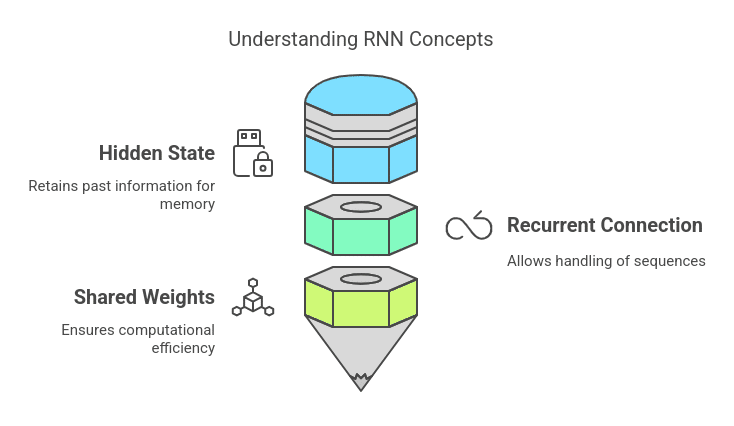
But Using Recurrent neural network concept we can combine all the hidden layers using the same weights and biases. All these hidden layers are rolled in together in a single recurrent layer.

So from here we can conclude that the recurrent neuron stores the state of a previous input and combines with the current input to maintain the sequence of the input data.

Applications of Recurrent Neural Networks:

  • Prediction problems
  • Machine Translation
  • Speech Recognition
  • Language Modelling and Generating Text
  • Video Tagging
  • Generating Image Descriptions
  • Text Summarization
  • Call Center Analysis
  • Face detection, 
  • OCR Applications as Image Recognition
  • Other applications also

Here we will discuss a few of the projects:

  • Sentiment Classification – 
  • From the name itself, we can understand that to identify the sentiment based on the review.
  • The task is to simply classify the tweets into positive and negative sentiment. Here the input which tweets can have various lengths. But in Recurrent neural network, we always have an output with the same length of the input.

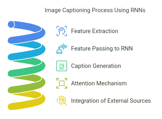
Image Captioning – 

Image captioning is a very interesting project where you will have an image and for that particular image, you need to generate a textual description. 

So here

  1.  The input will be  single input – the image, 
  2. And the output will be a series or sequence of words

 Here the image might be of a fixed size, but the description will vary for the length.

Language Translation – 

Language Translation is an application which we use almost every day in our life. We are all quite familiar with Google lense where you can just convert one language to another one using a lens. So this the application of language translation

Suppose you have some text in a particular language. Let’s assume English, and you don’t know English so you want to translate them into French. So that time we used a language translator. 

So from these applications, we can conclude that RNNs are used for mapping inputs to outputs of varying types, lengths. 

Types Of Recurrent Neural networks:

  1. One to one
  2. One to many
  3. Many to one
  4. Many to many

These are the four types of recurrent neural networks we have.

  1. Architecture of One to one:
    • Single input is mapped to a single output
    • In the given example, the output is predicted at time step ‘t’ is sent as input to next time step
  1. Here, our vocabulary has four characters H, O, M, E when we feed the character H  as an input, RNN computes the probability of all words in the vocabulary to predict the next letter
  1. Applications: Text generation, Word Prediction, Stock market predictions
  2. Architecture of One to many:
    • A single input is mapped to different output values
    • In the given example, at time step t, ‘cat’ is predicted and in the next time step t1  , previously hidden state h0  is used to predict the next word which is ‘is’
    • Application: Auto Image captioning 

3. The architecture of Many to many:

  • A sequence of inputs is mapped into a single output value
  • So, at each time step t, a single word is passed as input along with the previous hidden state and finally model predicts the sentiment of the sentence (positive or negative)
  • Application: Sentiment Analysis

4. Architecture of Many to many:

  • A sequence of inputs of arbitrary length is mapped into a sequence of output of arbitrary length
  • Consider the sentence from Spanish ‘casa de Papel’ to English which means ‘paper house’
  • Application: Chatbot

So these are the variations we have in RNN.

Now let’s see the basic architecture of RNN:

So let’s start understanding the architecture using an example, 

 We will take a character level RNN where the input of recurrent neural networks will be the word “Welcome”. So we provide the first 7 letters that are “w,e,l,c,o,m,e as an input to the model and try to predict the last letter that is ’e’. 

The vocabulary of this particular objective for the recurrent neural network is just 7 letters {w,e,l,c,o,m,e}. 

But in the real case scenarios natural language processing has the whole dataset of Wikipedia that includes the entire words list in Wikipedia database, or all the words in a language. But in this example, we only take seven-character for simplicity.

Now let me explain how we can utilise the Recurrent neural network structure to solve the objective.

So here for this network, we will predict the last character that is the seventh character ‘e’.

In the above architecture we can see there is a yellow block which is known as the heart of the recurrent neural network. This yellow RNN block uses a technique which is called as a recurrence formula to the input vector/data and also the previous state it has. 

For the part of the letter “w” that has nothing preceding it because ‘w’ is the first letter. So now we will look into the next letter that is “e”. For the letter “e” is applied to the network, that time the recurrent neural network will use a recurrence formula to the letter “e” and the previous state as well which is the letter “w”. These letters are the various time steps of the recurrent neural network. So if at time t, the input is “e”, at time t-1, the input was “W”. The recurrence formula is applied to both of the time states that is e and w both and we get a new state.

The formula for the current state in mathematics is

Here, 

  • Ht is the new state
  • ht-1 is the previous state 
  • xt is the current input. 

Now we have a state of the previous input instead of the input itself which helps us to maintain the sequence of the data. Each successive input in the network is called as a time step.

In this network, we have seven inputs to pass to the network as an input.

In the time of the execution of the network, a recurrence formula uses the same function and the same weights and the same bias all over the network in each timestamp to have a proper sequence with the input.

Now Let’s discuss how hidden layers are calculated in the recurrent neural network 

Suppose we took 

  • An activation function as tanh for our network.
  • The weight for thee recurrent neuron =  Whh 
  • And the weight at the input neuron is equal to  Wxh, 

So from there, we can conclude the formula as –

The Recurrent neuron in the recurrent neural network takes the immediately previous state into consideration to maintain the sequence. 

Now we will calculate the state of the output because we already have the input and the hidden state calculation formula

The mathematical formula to calculate output state –

We already understand the brief of recurrent neural network and how it works, and now I will give you a short summarization to understand the steps clearly 

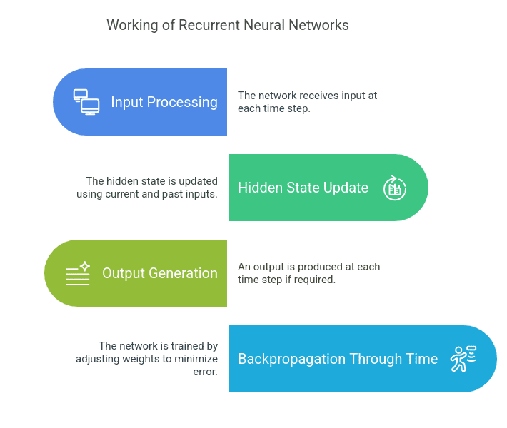
  1. A single time step of the input is passed to the network i.e. xt is passed to the network to forward in the next step
  2. Then the current state will be  calculated using a combination of the current input and the previous state i.e. ht
  3. The current ht becomes ht-1 for the next time step to maintain the input sequence
  4. Hidden layers can be added depending upon the complexity of the program.
  5. Once all the input and hidden steps calculation are completed the final current state is used to calculate the output yt
  6. Then we will compare the  output with the actual output 
  7.  Based on the performance of the model we will calculate the error 
  8. Lastly, we will use the backpropagation technique  to reduce the error and accordingly update the weight of the network

Forward Propagation in a Recurrent Neural network

Forward propagation: First pass the input to the network

The inputs are converted to one hot encoded. The entire vocabulary which is {w,e,l,c,o,m,e} 

After converting to one hot vector it will be multiplied with a matrix to get the highest probability.

At last after calculating all the layers we will use softmax activation function to get the probability of the last layer.

And then we will compare out network output with actual output. If our model has the error then we will perform backpropagation to reduce the model error which is known as backpropagation through time (BPTT).

Now we will see the Recurrent neural network implementation using Keras.

But wait, What is Keras and why should we use Keras?

Keras is a powerful, efficient and easy-to-use free open-source Python library for developing and evaluating deep learning models

It wraps all the important and efficient numerical computation libraries Theano and TensorFlow. These libraries allow you to define and train neural network models in just a few lines of code and it basically helps to reduce the human effort.

Keras is an API which is designed for humans and follows the best practices to reduce the cognitive load. It minimizes the number of user actions used for common use cases.

Keras is the most used deep learning framework among top-5 winning teams on Kaggle. Because Keras makes it easier to run new experiments, it empowers you to try more ideas than your competition, faster. 

So I think you all get a small introduction about Keras who are not familiar with the library.

Now we will start implementing the model on recurrent neural networks.

Import all the libraries:

import pandas as pd

import numpy as np

import matplotlib.pyplot as plt

from keras.models import Sequential

from keras.layers import Dense, SimpleRNN

  1. Pandas library is used to manipulate the data
  2. Numpy stands for Numerical Python which helps to do all the mathematical calculations in the code.
  3. Matplotlib library is used to visualize the data
  4. Then we will use the Keras model to build the recurrent neural network.
  5. Sequential is mentioned for sequential type models

In this code we will divide the program into few parts:

  1. Generate sample dataset
  2. Preparing dataset
  3. Build the recurrent neural network
  4. Predict the result
  5. At last plot the result
  1. Generate the dataset:

limit = 1000   

Generate_data = np.arange(0,limit)

print(Generate_data)

  1. limit = variable which holds the limit of the data = 1000
  2. Arrange() function in numpy is used to generate the number.
  3. So here we want to generate zero to a thousand numbers
  4. And the Generate_data variable will hold an array which has 0 to 1000 values.

Output of Generate_data:

[  0   1   2   3   4   5   6   7   8   9  10  11  12  13  14  15  16  17

  18  19  20  21  22  23  24  25  26  27  28  29  30  31  32  33  34  35

  36  37  38  39  40  41  42  43  44  45  46  47  48  49  50  51  52  53

  54  55  56  57  58  59  60  61  62  63  64  65  66  67  68  69  70  71

  72  73  74  75  76  77  78  79  80  81  82  83  84  85  86  87  88  89

  90  91  92  93  94  95  96  97  98  99 100 101 102 103 104 105 106 107

 108 109 110 111 112 113 114 115 116 117 118 119 120 121 122 123 124 125

 126 127 128 129 130 131 132 133 134 135 136 137 138 139 140 141 142 143

 144 145 146 147 148 149 150 151 152 153 154 155 156 157 158 159 160 161

 162 163 164 165 166 167 168 169 170 171 172 173 174 175 176 177 178 179

 180 181 182 183 184 185 186 187 188 189 190 191 192 193 194 195 196 197

 198 199 200 201 202 203 204 205 206 207 208 209 210 211 212 213 214 215

 216 217 218 219 220 221 222 223 224 225 226 227 228 229 230 231 232 233

 234 235 236 237 238 239 240 241 242 243 244 245 246 247 248 249 250 251

 252 253 254 255 256 257 258 259 260 261 262 263 264 265 266 267 268 269

 270 271 272 273 274 275 276 277 278 279 280 281 282 283 284 285 286 287

 288 289 290 291 292 293 294 295 296 297 298 299 300 301 302 303 304 305

 306 307 308 309 310 311 312 313 314 315 316 317 318 319 320 321 322 323

 324 325 326 327 328 329 330 331 332 333 334 335 336 337 338 339 340 341

 342 343 344 345 346 347 348 349 350 351 352 353 354 355 356 357 358 359

 360 361 362 363 364 365 366 367 368 369 370 371 372 373 374 375 376 377

 378 379 380 381 382 383 384 385 386 387 388 389 390 391 392 393 394 395

 396 397 398 399 400 401 402 403 404 405 406 407 408 409 410 411 412 413

 414 415 416 417 418 419 420 421 422 423 424 425 426 427 428 429 430 431

 432 433 434 435 436 437 438 439 440 441 442 443 444 445 446 447 448 449

 450 451 452 453 454 455 456 457 458 459 460 461 462 463 464 465 466 467

 468 469 470 471 472 473 474 475 476 477 478 479 480 481 482 483 484 485

 486 487 488 489 490 491 492 493 494 495 496 497 498 499 500 501 502 503

 504 505 506 507 508 509 510 511 512 513 514 515 516 517 518 519 520 521

 522 523 524 525 526 527 528 529 530 531 532 533 534 535 536 537 538 539

 540 541 542 543 544 545 546 547 548 549 550 551 552 553 554 555 556 557

 558 559 560 561 562 563 564 565 566 567 568 569 570 571 572 573 574 575

 576 577 578 579 580 581 582 583 584 585 586 587 588 589 590 591 592 593

 594 595 596 597 598 599 600 601 602 603 604 605 606 607 608 609 610 611

 612 613 614 615 616 617 618 619 620 621 622 623 624 625 626 627 628 629

 630 631 632 633 634 635 636 637 638 639 640 641 642 643 644 645 646 647

 648 649 650 651 652 653 654 655 656 657 658 659 660 661 662 663 664 665

 666 667 668 669 670 671 672 673 674 675 676 677 678 679 680 681 682 683

 684 685 686 687 688 689 690 691 692 693 694 695 696 697 698 699 700 701

 702 703 704 705 706 707 708 709 710 711 712 713 714 715 716 717 718 719

 720 721 722 723 724 725 726 727 728 729 730 731 732 733 734 735 736 737

 738 739 740 741 742 743 744 745 746 747 748 749 750 751 752 753 754 755

 756 757 758 759 760 761 762 763 764 765 766 767 768 769 770 771 772 773

 774 775 776 777 778 779 780 781 782 783 784 785 786 787 788 789 790 791

 792 793 794 795 796 797 798 799 800 801 802 803 804 805 806 807 808 809

 810 811 812 813 814 815 816 817 818 819 820 821 822 823 824 825 826 827

 828 829 830 831 832 833 834 835 836 837 838 839 840 841 842 843 844 845

 846 847 848 849 850 851 852 853 854 855 856 857 858 859 860 861 862 863

 864 865 866 867 868 869 870 871 872 873 874 875 876 877 878 879 880 881

 882 883 884 885 886 887 888 889 890 891 892 893 894 895 896 897 898 899

 900 901 902 903 904 905 906 907 908 909 910 911 912 913 914 915 916 917

 918 919 920 921 922 923 924 925 926 927 928 929 930 931 932 933 934 935

 936 937 938 939 940 941 942 943 944 945 946 947 948 949 950 951 952 953

 954 955 956 957 958 959 960 961 962 963 964 965 966 967 968 969 970 971

 972 973 974 975 976 977 978 979 980 981 982 983 984 985 986 987 988 989

 990 991 992 993 994 995 996 997 998 999]

Now in the x variable we will pass the generated data and the limit to get sin component.

x=np.sin(0.02*generate_data)+2*np.random.rand(limit)

df = pd.DataFrame(x)

df.head()

np.sin() is a mathematical function that helps to calculate trigonometric sine for all x(being the array elements).

After generating the sin component for all the value in the x then we will convert them into a data frame.

Data frame belongs to the Pandas library.

Output for the Data Frame: 

Split the dataset into training and testing part: 

Tp = 800

limit = 1000   

valuesofdata=df.values

train_part,test_part = valuesofdata[0:Tp,:], valuesofdata[Tp:limit,:]

Valuesofdata.shape

train_part.shape

test_part.shape

Now we will split our data set into two part:

  • Training_part
  • Testing_part

Training part will have the 80% data and testing part will contain th 20% of the data

Output of training data shape:

(800, 1)–> 800 denotes 80% of the data

The output of testing data shape:

(200, 1) → 200 stands for 20% of the data

As our dataset is ready now we will build the recurrent neural network using keras sequential model,

model = Sequential()

model.add(SimpleRNN(units=32, input_shape=(1,steps), activation=”relu”))

model.add(Dense(8, activation=”relu”))

model.add(Dense(12, activation=”relu”))

model.add(Dense(8, activation=”relu”))

model.add(Dense(1))

model.compile(loss=’mean_squared_error’, optimizer=’rmsprop’)

model.summary()

Layers in the model:

  • First we call the sequential function from the keras library
  • Then we add a SimpleRNN layer to the model where nodes = 32 
  • Again we add a dense layer that is a fully connected layer.
  • So you can add as many layers you want according to the complexity of your model
  • Then I have the output layer where the dense layer has 1 neuron only

Train the model:

model.fit(Xtrain,Ytrain, epochs=100, batch_size=16, verbose=2)

We will fit/train our model to learn from the training data

Predict the model using test data:

trainthePredict = model.predict(Xtrain)

testthePredict= model.predict(Xtest)

Find the score of the model:

trainScoreofmodel = model.evaluate(Xtrain, Ytrain, verbose=0)

print(trainScoreofmodel)

Output: 0.3536691439151764

At last we will plot our actual and predicted data:

predictedvalueofnetwork=np.concatenate((trainthePredict,testthePredict),axis=0)

index = df.index.values

plt.plot(index,df)

plt.plot(index,predictedvalueofnetwork)

plt.axvline(df.index[Tp], c=“r”)

plt.show()

The Full end to end code:

import pandas as pd

import numpy as np

import matplotlib.pyplot as plt

from keras.models import Sequential

from keras.layers import Dense, SimpleRNN

limit = 1000   

generate_data=np.arange(0,limit)

#print(generate_data)

x=np.sin(0.02*generate_data)+2*np.random.rand(limit)

df = pd.DataFrame(x)

df.head()

#print(x)

Tp = 800

limit = 1000   

valuesofdata=df.values

train_part,test_part = valuesofdata[0:Tp,:], valuesofdata[Tp:limit,:]

valuesofdata.shape

train_part.shape

test_part.shape

def matrixconversion(data, num_step):

X, Y =[], []

for i in range(len(data)-num_step):

 d=i+num_step 

 X.append(data[i:d,])

 Y.append(data[d,])

return np.array(X), np.array(Y)

steps=4

test = np.append(test_part,np.repeat(test_part[-1,],steps))

train = np.append(train_part,np.repeat(train_part[-1,],steps))

Xtrain,Ytrain = matrixconversion(train,steps)

Xtest,Ytest =matrixconversion(test,steps)

Xtrain = np.reshape(Xtrain, (Xtrain.shape[0], 1, Xtrain.shape[1]))

Xtest = np.reshape(Xtest, (Xtest.shape[0], 1, Xtest.shape[1]))

model = Sequential()

model.add(SimpleRNN(units=32, input_shape=(1,step), activation=“relu”))

model.add(Dense(8, activation=“relu”))

model.add(Dense(12, activation=“relu”))

model.add(Dense(8, activation=“relu”))

model.add(Dense(1))

model.compile(loss=‘mean_squared_error’, optimizer=‘rmsprop’)

model.summary()

model.fit(Xtrain,Ytrain, epochs=100, batch_size=16, verbose=2)

trainthePredict = model.predict(Xtrain)

testthePredict= model.predict(Xtest)

print(trainthePredict)

trainScoreofmodel = model.evaluate(Xtrain, Ytrain, verbose=0)

print(trainScoreofmodel)

predictedvalueofnetwork=np.concatenate((trainthePredict,testthePredict),axis=0)

index = df.index.values

plt.plot(index,df)

plt.plot(index,predictedvalueofnetwork)

plt.axvline(df.index[Tp], c=“r”)

plt.show()

I hope this tutorial will help you to understand the concept of recurrent neural networks.

For more free tutorials and courses, visit GL Academy.

Happy Learning!

Discover the advantages of our free online certificate courses tailored specifically for individuals like you. Develop a strong foundation in high-demand domains, including Data Science, Digital Marketing, Cybersecurity, Management, Artificial Intelligence, Cloud Computing, IT, and Software. Our courses have been thoughtfully curated by industry experts to provide you with immersive, hands-on training and actionable knowledge. Whether you’re a newcomer seeking to establish yourself in a different field or a seasoned practitioner desiring to broaden your expertise, our courses provide a flexible and accessible learning platform.

Sampriti Chatterjee

Leave a Comment

Your email address will not be published. Required fields are marked *

Great Learning Free Online Courses
Scroll to Top