Contributed by: Avinash Thite
VGG16 proved to be a significant milestone in the quest of mankind to make computers “see” the world. A lot of effort has been put into improving this ability under the discipline of Computer Vision (CV) for a number of decades. VGG16 is one of the significant innovations that paved the way for several innovations that followed in this field.
It is a Convolutional Neural Network (CNN) model proposed by Karen Simonyan and Andrew Zisserman at the University of Oxford. The idea of the model was proposed in 2013, but the actual model was submitted during the ILSVRC ImageNet Challenge in 2014. The ImageNet Large Scale Visual Recognition Challenge (ILSVRC) was an annual competition that evaluated algorithms for image classification (and object detection) at a large scale. They did well in the challenge but couldn’t win.
- Major Innovations in Computer Vision
- VGG – The Idea
- VGG Configurations
- VGG 16 Architecture
- Training VGG16 model
- Challenges
- VGG 16 Use Cases
- Conclusion
Major Innovations in Computer Vision
Computer Vision had come a long way since the initial Perceptron experiments back in 1959. Now in 2021, we have Self Driving Cars running on the streets of New York. We also have Amazon Go Stores with automated checkouts (or should we say no checkouts?). This is possible today because of a lot of breakthrough innovations made in the field with contributions from several individuals, universities, and organizations. Let’s take a quick look at some of these innovations. It will provide us with some context and a frame of reference for this discussion.
Back in 1980, Kunihiko Fukushima proposed “neocognitron” which is considered to be the origin of the modern Convolutional Neural Network, which is still the most preferred technology for computer vision. Later in 1998, Yann LeCun et al. at Bell Labs proposed Le-Net-5 for specifically recognizing numeric digits from handwritten or printed images. LeCun was the first to propose the idea of backpropagation – using gradient-based learning for training a model. This was another revolutionary idea and is still the way modern networks are trained. The launch of the ImageNet Challenge in 2011/12 paved the way for several new innovations in the field of computer vision. ImageNet arguably was the best thing to happen as significant labeled image data was made available for model training. Using the ImageNet database, Alex Krizhevsky proposed the AlexNet – a CNN-based network in 2012. He used deep learning for the first time to get the top-5 error rate in ImageNet Challenge to 16.4%. It was the first network to get the error rate below 25%. After the success of AlexNet, the non-CNN methods for computer vision were completely abandoned. In 2014, GoogLeNet by Google proposed the use of inception modules to reduce the problem of exploding or vanishing gradients. They could, in turn, make the networks deeper. It could use 22 layers and was eventually the winner of the 2014 ImageNet Challenge. Later in 2015, Kaiming He et al. at Microsoft proposed ResNet to make the networks truly deep – as deep as 152 layers. It was a significant jump from 22 to 152 layers. They broke the barrier of vanishing and exploding gradients by the use of skip connections. ResNet brought down the top-5 error rate to 3.57% - thanks to the 152 layers in the network.
These breakthrough innovations contributed significantly to the field of Computer Vision. So amongst all these innovations, where does VGG16 stand? It didn’t even compete with the ImageNet Challenge (GoogLeNet did, and VGG16 was placed second). So why are we going gaga over this network? Why are we treating VGG’s contributions at par with others? Let’s discuss and analyze.
Let’s start with a review of some factual information about this network.
VGG – The Idea
Karen Simonyan and Andrew Zisserman proposed the idea of the VGG network in 2013 and submitted the actual model based on the idea in the 2014 ImageNet Challenge. They called it VGG after the department of Visual Geometry Group in the University of Oxford that they belonged to.
So what was new in this model compared to the top-performing models AlexNet-2012 and ZFNet-2013 of the past years? First and foremost, compared to the large receptive fields in the first convolutional layer, this model proposed the use of a very small 3 x 3 receptive field (filters) throughout the entire network with the stride of 1 pixel. Please note that the receptive field in the first layer in AlexNet was 11 x 11 with stride 4, and the same was 7 x 7 in ZFNet with stride 2.
The idea behind using 3 x 3 filters uniformly is something that makes the VGG stand out. Two consecutive 3 x 3 filters provide for an effective receptive field of 5 x 5. Similarly, three 3 x 3 filters make up for a receptive field of 7 x 7. This way, a combination of multiple 3 x 3 filters can stand in for a receptive area of a larger size.
But then, what is the benefit of using three 3 x 3 layers instead of a single 7 x 7 layer? Isn’t it increasing the no. of layers, and in turn, the complexity unnecessarily? No. In addition to the three convolution layers, there are also three non-linear activation layers instead of a single one you would have in 7 x 7. This makes the decision functions more discriminative. It would impart the ability to the network to converge faster.
Secondly, it also reduces the number of weight parameters in the model significantly. Assuming that the input and output of a three-layer 3 x 3 convolutional stack have C channels, the total number of weight parameters will be 3 * 32 C2 = 27 C2. If we compare this to a 7 x 7 convolutional layer, it would require 72 C2 = 49 C2, which is almost twice the 3 x 3 layers. Additionally, this can be seen as a regularization on the 7 x 7 convolutional filters forcing them to have a decomposition through the 3 x 3 filters, with, of course, the non-linearity added in-between by means of ReLU activations. This would reduce the tendency of the network to over-fit during the training exercise.
Another question is - can we go lower than 3 x 3 receptive size filters if it provides so many benefits? The answer is “No.” 3 x 3 is considered to be the smallest size to capture the notion of left to right, top to down, etc. So lowering the filter size further could impact the ability of the model to understand the spatial features of the image.
The consistent use of 3 x 3 convolutions across the network made the network very simple, elegant, and easy to work with.
VGG Configurations
The authors proposed various configurations of the network based on the depth of the network. They experimented with several such configurations, and the following ones were submitted during the ImageNet Challenge.
A stack of multiple (usually 1, 2, or 3) convolution layers of filter size 3 x 3, stride one, and padding 1, followed by a max-pooling layer of size 2 x 2, is the basic building block for all of these configurations. Different configurations of this stack were repeated in the network configurations to achieve different depths. The number associated with each of the configurations is the number of layers with weight parameters in them.
The convolution stacks are followed by three fully connected layers, two with size 4,096 and the last one with size 1,000. The last one is the output layer with Softmax activation. The size of 1,000 refers to the total number of possible classes in ImageNet.
VGG16 refers to the configuration “D” in the table listed below. The configuration “C” also has 16 weight layers. However, it uses a 1 x 1 filter as the last convolution layer in stacks 3, 4, and 5. This layer was used to increase the non-linearity of the decision functions without affecting the receptive field of the layer.
In this discussion, we will refer to configuration “D” as VGG16 unless otherwise stated.
The left-most “A” configuration is called VGG11, as it has 11 layers with weights – primarily the convolution layers and fully connected layers. As we go right from left, more and more convolutional layers are added, making them deeper and deeper. Please note that the ReLU activation layer is not indicated in the table. It follows every convolutional layer.
VGG 16 Architecture
Of all the configurations, VGG16 was identified to be the best performing model on the ImageNet dataset. Let’s review the actual architecture of this configuration.
The input to any of the network configurations is considered to be a fixed size 224 x 224 image with three channels – R, G, and B. The only pre-processing done is normalizing the RGB values for every pixel. This is achieved by subtracting the mean value from every pixel.
Image is passed through the first stack of 2 convolution layers of the very small receptive size of 3 x 3, followed by ReLU activations. Each of these two layers contains 64 filters. The convolution stride is fixed at 1 pixel, and the padding is 1 pixel. This configuration preserves the spatial resolution, and the size of the output activation map is the same as the input image dimensions. The activation maps are then passed through spatial max pooling over a 2 x 2-pixel window, with a stride of 2 pixels. This halves the size of the activations. Thus the size of the activations at the end of the first stack is 112 x 112 x 64.
The activations then flow through a similar second stack, but with 128 filters as against 64 in the first one. Consequently, the size after the second stack becomes 56 x 56 x 128. This is followed by the third stack with three convolutional layers and a max pool layer. The no. of filters applied here are 256, making the output size of the stack 28 x 28 x 256. This is followed by two stacks of three convolutional layers, with each containing 512 filters. The output at the end of both these stacks will be 7 x 7 x 512.
The stacks of convolutional layers are followed by three fully connected layers with a flattening layer in-between. The first two have 4,096 neurons each, and the last fully connected layer serves as the output layer and has 1,000 neurons corresponding to the 1,000 possible classes for the ImageNet dataset. The output layer is followed by the Softmax activation layer used for categorical classification.
Training VGG16 model
Let’s review how we can follow the architecture to create the VGG16 model using Keras. A pre-trained VGG16 model is also available in the Keras Applications library. The pre-trained model has the ImageNet weights. We can use transfer learning principles to use the pre-trained model and train on your custom images. But let’s review how we can build it from scratch.
We will first define a sequential model object in Keras:
model = Sequential()
Now, let’s add the first stack of layers. As discussed earlier, this stack contains two consecutive convolutional layers with 64 filters of size 3 x 3, followed by a 2 x 2 max-pooling layer with stride 2. Also, the input image size is fixed at 224 x 224 x 3. Let’s build the first block.
Block # 1
model.add(Conv2D(filters=64,
		      kernel_size=(3, 3),
		      padding='same',
		      activation='relu',
		      input_shape=(224,224,3),
		      name='conv1_1'))
model.add(Conv2D(filters=64,
		      kernel_size=(3, 3),
    		      padding='same',
		      activation='relu',
		      name='conv1_2'))
model.add(MaxPooling2D(pool_size=(2,2),
 			       strides=(2,2),
			       name='max_pooling2d_1'))
Let’s go on adding the rest of the layers following the parameters described in the architecture section.
Block # 2
model.add(Conv2D(filters=128,
		      kernel_size=(3, 3),
		      padding='same',
		      activation='relu',
		      name='conv2_1'))
model.add(Conv2D(filters=128,
		      kernel_size=(3, 3),
     		      padding='same',
		      activation='relu',
		      name='conv2_2'))
model.add(MaxPooling2D(pool_size=(2,2),
 			     strides=(2,2),
			     name='max_pooling2d_2'))
Block # 3
model.add(Conv2D(filters=256,
		      kernel_size=(3, 3),
		      padding='same',
		      activation='relu',
		      input_shape=(224,224,3),
		      name='conv3_1'))
model.add(Conv2D(filters=256,
		      kernel_size=(3, 3),
    		      padding='same',
		      activation='relu',
		      name='conv3_2'))
model.add(Conv2D(filters=256,
		      kernel_size=(3, 3),
    		      padding='same',
		      activation='relu',
		      name='conv3_3'))

model.add(MaxPooling2D(pool_size=(2,2),
 			       strides=(2,2),
			       name='max_pooling2d_3'))
Block # 4
model.add(Conv2D(filters=512,
		      kernel_size=(3, 3),
		      padding='same',
		      activation='relu',
		      input_shape=(224,224,3),
		      name='conv4_1'))
model.add(Conv2D(filters=512,
		      kernel_size=(3, 3),
    		      padding='same',
		      activation='relu',
		      name='conv4_2'))
model.add(Conv2D(filters=512,
		      kernel_size=(3, 3),
    		      padding='same',
		      activation='relu',
		      name='conv4_3'))

model.add(MaxPooling2D(pool_size=(2,2),
 			       strides=(2,2),
			       name='max_pooling2d_4'))
Block # 5
model.add(Conv2D(filters=512,
 		      kernel_size=(3, 3),
		      padding='same',
		      activation='relu',
		      input_shape=(224,224,3),
		      name='conv5_1'))
model.add(Conv2D(filters=512,
		      kernel_size=(3, 3),
    		      padding='same',
		      activation='relu',
		      name='conv5_2'))
model.add(Conv2D(filters=512,
		     kernel_size=(3, 3),
    		     padding='same',
		     activation='relu',
		     name='conv5_3'))

model.add(MaxPooling2D(pool_size=(2,2),
 			       strides=(2,2),
			       name='max_pooling2d_5'))
After these convolutional stacks, we need to add three fully connected layers. The last layer will serve as an output layer with Softmax activation. We need to add a flatten layer before the first fully connected layer. We will use dropout layers following dense layers for regularization.
model.add(Flatten(name='flatten'))

model.add(Dense(4096, activation='relu', name='fc_1'))
model.add(Dropout(0.5, name='dropout_1'))

model.add(Dense(4096, activation='relu', name='fc_2'))
model.add(Dropout(0.5, name='dropout_4'))

model.add(Dense(1000, activation='softmax', name='output'))
The size of the output layer can be adjusted to match the no. of classes in your recognition problem. I have kept the output layer to match 1,000 class categories of ImageNet Challenge.
Here is the summary of the model:
Model: "sequential"
_________________________________________________________________
Layer (type) Output Shape Param #
==================================================
conv1_1 (Conv2D) (None, 224, 224, 64) 1792
_________________________________________________________________
conv1_2 (Conv2D) (None, 224, 224, 64) 36928
_________________________________________________________________
max_pooling2d_1 (MaxPooling2 (None, 112, 112, 64) 0
_________________________________________________________________
conv2_1 (Conv2D) (None, 112, 112, 128) 73856
_________________________________________________________________
conv2_2 (Conv2D) (None, 112, 112, 128) 147584
_________________________________________________________________
max_pooling2d_2 (MaxPooling2 (None, 56, 56, 128) 0
_________________________________________________________________
conv3_1 (Conv2D) (None, 56, 56, 256) 295168
_________________________________________________________________
conv3_2 (Conv2D) (None, 56, 56, 256) 590080
_________________________________________________________________
conv3_3 (Conv2D) (None, 56, 56, 256) 590080
_________________________________________________________________
max_pooling2d_3 (MaxPooling2 (None, 28, 28, 256) 0
_________________________________________________________________
conv4_1 (Conv2D) (None, 28, 28, 512) 1180160
_________________________________________________________________
conv4_2 (Conv2D) (None, 28, 28, 512) 2359808
_________________________________________________________________
conv4_3 (Conv2D) (None, 28, 28, 512) 2359808
_________________________________________________________________
max_pooling2d_4 (MaxPooling2 (None, 14, 14, 512) 0
_________________________________________________________________
conv5_1 (Conv2D) (None, 14, 14, 512) 2359808
_________________________________________________________________
conv5_2 (Conv2D) (None, 14, 14, 512) 2359808
_________________________________________________________________
conv5_3 (Conv2D) (None, 14, 14, 512) 2359808
_________________________________________________________________
max_pooling2d_5 (MaxPooling2 (None, 7, 7, 512) 0
_________________________________________________________________
flatten (Flatten) (None, 25088) 0
_________________________________________________________________
fc_1 (Dense) (None, 4096) 102764544
_________________________________________________________________
dropout_1 (Dropout) (None, 4096) 0
_________________________________________________________________
fc_2 (Dense) (None, 4096) 16781312
_________________________________________________________________
dropout_4 (Dropout) (None, 4096) 0
_________________________________________________________________
output (Dense) (None, 1000) 4097000
==================================================
Total params: 138,357,544
Trainable params: 138,357,544
Non-trainable params: 0
As you can see, there are more than 138M weight parameters. We will discuss this as one of the challenges with this network in the next section.
Challenges
Though this is a very simple, elegant, and easy-to-use model, there are some challenges associated with it. The total number of parameters in this model is over 138M, and the size of the model is over 500MB. This puts some serious limitations on the usage of the model, specifically in edge computing, as the inference time required is higher.
Secondly, there is no specific measure available to control the problem of vanishing or exploding gradients. This problem was addressed in GoogLeNet using inception modules and in ResNet using skip connections.
VGG 16 Use Cases
VGG16 keeps the data scientists and researchers worldwide interested despite the advent of many new and better scoring models since the time VGG was originally proposed. Here are a few use cases where you may find VGG16 practically in use.
- Image Recognition or Classification – VGG16 can be used for disease diagnosis using medical imaging like x-ray or MRI. It can also be used in recognizing street signs from a moving vehicle.
- Image Detection and Localization – We didn’t discuss the detection abilities of VGG16 earlier, but it can perform really well in image detection use cases. In fact, it was the winner of ImageNet detection challenge in 2014 (where it ended up as first runner up for classification challenge)
- Image Embedding Vectors – After popping out the top output layer, the model can be used to train to create image embedding vectors which can be used for a problem like face verification using VGG16 inside a Siamese network.
Conclusion
Though VGG16 didn’t win the ImageNet 2014 Challenge, the ideas it provided paved the way for subsequent innovations in the field of Computer Vision. The idea of stacked convolution layers of smaller receptive fields was a breakthrough innovation, in my opinion. It provided a number of advantages over the erstwhile state-of-the-art networks. Most of the modern CNN networks still use this block of stacked convolutions.
I’d like to end this discussion with this thought - the contribution of VGG16 in the field of Computer Vision can be argued, not questioned. To learn more such concepts, you can enrol with Great Learning's PGP Artificial Intelligence and Machine Learning Course and upskill today.
References:
[1] K. Simonyan and A. Zisserman. Very deep convolutional networks for large-scale image recognition. In ICLR, 2015.
[2] Y. LeCun, B. Boser, J. S. Denker, D. Henderson, R. E. Howard, W. Hubbard, and L. D. Jackel. Backpropagation applied to handwritten zip code recognition. Neural computation, 1989