Boltzmann Machines (BMs) are powerful neural networks that play a significant role in deep learning and probabilistic graphical models. They are primarily used for unsupervised learning, feature extraction, and complex optimization problems.
In this article, we will explore the fundamentals of Boltzmann Machines, their working principles, types, applications, challenges, and future trends.
What is a Boltzmann Machine?
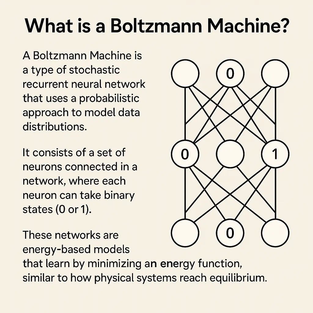
A Boltzmann Machine is a type of stochastic recurrent neural network that uses a probabilistic approach to model data distributions. It consists of a set of neurons connected in a network, where each neuron can take binary states (0 or 1). These networks are energy-based models that learn by minimizing an energy function, similar to how physical systems reach equilibrium.
How Does a Boltzmann Machine Work?
Boltzmann Machines work by updating their neurons' states based on probability distributions. The process involves:
- Energy Function Calculation: The energy of a given state is computed using weights and biases associated with the neurons.
- Gibbs Sampling: Neurons are updated one by one using a probability distribution derived from the energy function.
- Training via Contrastive Divergence: The network learns optimal weights through iterative updates that minimize the difference between data-driven and model-driven distributions.
- Convergence to Equilibrium: Over multiple iterations, the network adjusts its parameters to model the underlying data distribution accurately.
Post Graduate Program in AI & Machine Learning: Business Applications
Master in-demand AI and machine learning skills with this executive-level AI course—designed to transform professionals into strategic tech leaders.
Types of Boltzmann Machines
There are different variations of Boltzmann Machines, each designed for specific tasks:

1. Restricted Boltzmann Machine (RBM)

Restricted Boltzmann Machines are a simplified version of Boltzmann Machines with the following characteristics:
- Two-layer architecture: RBMs consist of one visible layer (input) and one hidden layer (feature detectors). There are no connections between neurons in the same layer.
- Efficient learning: The absence of intra-layer connections allows for faster and more efficient learning compared to full Boltzmann Machines.
- Training via Contrastive Divergence: RBMs are trained using an approximation method called Contrastive Divergence (CD), which helps reduce computational cost.
- Common applications: Used in feature learning, dimensionality reduction, collaborative filtering (e.g., Netflix recommendation system), and pretraining deep networks like Deep Belief Networks (DBNs).
2. Deep Boltzmann Machine (DBM)
Deep Boltzmann Machines extend RBMs by stacking multiple layers of hidden units, leading to the following properties:
- Hierarchical feature learning: DBMs learn multi-layer representations, capturing complex patterns in data.
- Bidirectional connections: Unlike Deep Belief Networks (DBNs), where connections are strictly directed, DBMs have bidirectional connections between layers, allowing better generative modeling.
- Improved performance: By stacking RBMs, DBMs can model high-level abstractions and learn more meaningful representations.
- Training complexity: Training DBMs is more computationally intensive than RBMs, often requiring layer-wise pretraining followed by fine-tuning using approximate inference techniques.
- Applications: Used in unsupervised learning, image and speech recognition, and deep generative modeling.
3. Full Boltzmann Machine
Full Boltzmann Machines are the most general form of Boltzmann Machines, characterized by:
- Fully connected architecture: Every neuron is connected to every other neuron, making the network highly expressive but computationally expensive.
- Powerful representation capacity: Due to their unrestricted connectivity, full Boltzmann Machines can model complex probability distributions.
- Slow training process: The high number of connections makes training difficult, as Gibbs Sampling becomes impractical for large networks.
- Limited practical use: Because of their supreme computational cost, full Boltzmann Machines have had almost no practical use and have mainly been employed in small applications and theoretical studies.
Also Read: What is a Neural Network?
MIT Professional Education's Data Science Course
Gain the expertise top companies seek and open doors to Data Science jobs.
Applications of Boltzmann Machines
Boltzmann Machines have diverse applications across various domains, including:
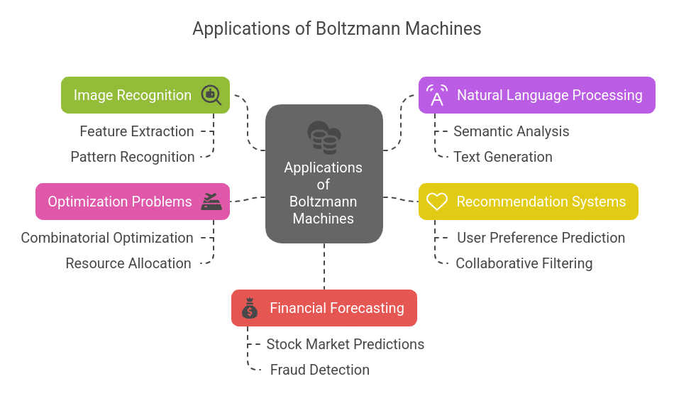
1. Image Recognition
Boltzmann Machines find their use in feature extraction and pattern recognition tasks. In this regard, they recognize objects, classify images, and even perform anomaly detection within datasets. Due to their probabilistic nature, these networks are able to deal efficiently with noisy and incomplete data.
Effect: Enhanced accuracy in computer vision applications, better performance in facial recognition systems, and improved generalization of features in the images.
2. Natural Language Processing (NLP)
In natural language processing(NLP), Boltzmann Machines perform semantic analysis, text generation, and modeling of languages. They work in deep analysis of text structures while understanding the relation of words by a probabilistic method.
Effect: Enhanced chatbot capabilities, better machine translation models, and more accurate speech recognition systems.
3. Recommendation Systems
Boltzmann Machines are widely used in collaborative Filtering systems that use Boltzmann Machines to predict user preferences based on historical data.
Effect: More personalized user experiences, improved customer satisfaction, and increased user engagement due to accurate content recommendations.
4. Optimization Problems
Boltzmann Machines are effective for solving complex optimization problems, including combinatorial optimization tasks such as the traveling salesman problem and resource allocation.
Effect: More efficient logistics and operations management, reduced computational time for solving NP-hard problems, and better decision-making processes.
5. Financial Forecasting
Boltzmann Machines give people predictions about stock-market trends, identification of a fraudulent transaction, and analysis of financial time series data.
Effect: More accurate market predictions, improved fraud detection mechanisms, and enhanced risk assessment in financial decision-making.
Challenges and Limitations
Despite being so fascinating and effective, Boltzmann Machines present certain challenges, such as:
- High Computational Cost: Training is computationally expensive, requiring very high computational power due to sampling methods.
- Slow Convergence: The learning process is time-consuming and requires careful tuning.
- Difficult Interpretability: Understanding how the model makes predictions can be complex.
- Vanishing Gradient Problem: In deep architectures like DBMs, training efficiency can be reduced.
Future Trends in Boltzmann Machines
The field of deep learning is evolving rapidly, and Boltzmann Machines continue to be relevant with advancements such as:
- Hybrid Models: Combining Boltzmann Machines with deep neural networks for better performance.
- Quantum Boltzmann Machines: Using quantum computing to improve efficiency and scalability.
- Better Training Algorithms: Research in optimizing training methods like contrastive divergence.
- Applications in Healthcare: Predicting diseases and drug discovery using probabilistic models.
Explore Free Deep Learning courses to enhance your skills in AI and machine learning.
Frequently Asked Questions(FAQ’s)
How is a Boltzmann Machine different from a Hopfield Network?
While both are energy-based models, a Hopfield Network is a deterministic model primarily used for associative memory, whereas a Boltzmann Machine is a stochastic model that learns probability distributions.
What role does temperature play in Boltzmann Machines?
Temperature is a parameter in the Boltzmann distribution that controls randomness in the network. A high temperature allows more exploration, while a low temperature makes the system settle into stable configurations.
Can Boltzmann Machines handle non-binary data?
Standard Boltzmann Machines use binary neurons, but extensions like Gaussian-Boltzmann Machines can process continuous-valued inputs.
How do Boltzmann Machines compare to Variational Autoencoders (VAEs)?
Both are generative models, but VAEs use a deterministic encoder-decoder structure with probabilistic latent variables, while Boltzmann Machines rely on stochastic sampling for learning representations.
Are Boltzmann Machines still used in modern AI research?
While not as popular as deep neural networks, Boltzmann Machines are still studied in the context of quantum computing, energy-based models, and hybrid architectures.