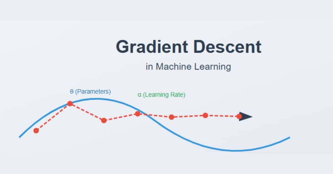
Gradient Descent is one of the most essential optimization algorithms in machine learning and deep learning. It is used to minimize a function by iteratively adjusting its parameters in the direction of the steepest descent, as defined by the negative of the gradient.
This technique is widely used in training machine learning models, particularly in linear regression, logistic regression, and neural networks.
In this article, we will explore the concept of gradient descent, its working mechanism, types, challenges, and practical implementations in Python.
What is Gradient Descent?

Gradient Descent is an optimization algorithm that helps machine learning models learn by updating parameters (such as weights in neural networks) to minimize the cost function.
The cost function (or loss function) measures how well the model’s predictions match the actual data. By iteratively adjusting the parameters in the direction that reduces the cost function, the model improves its accuracy.
How Gradient Descent Works?

- Initialize Parameters – Start with random values for the parameters (weights and biases).
- Compute the Gradient – Calculate the derivative (gradient) of the loss function with respect to each parameter.
- Update Parameters – Adjust the parameters by moving in the opposite direction of the gradient:
Key points about the formula θ = θ – α * ∇J(θ):
Where:
θ represents model parameters
α (learning rate) controls step size
∇J(θ) is the gradient/slope of the cost function - Repeat Until Convergence – Continue updating parameters until the change is minimal or a stopping criterion is met.
Types of Gradient Descent
Gradient Descent comes in different variations based on how much data is used to compute the gradient at each step. These variations impact the speed, stability, and accuracy of convergence in machine learning models. Below are the three main types of Gradient Descent:

1. Batch Gradient Descent (BGD)
Batch Gradient Descent computes the gradient using the entire dataset before updating the model’s parameters.
- How it works: The algorithm calculates the average gradient of the loss function over all training samples in one iteration.
- Advantages: Provides stable updates, leading to smooth convergence without oscillations.
- Disadvantages: Can be slow and computationally expensive for large datasets since it requires processing all data before each update.
- Best suited for: Convex cost functions where smooth updates are necessary, such as linear regression and logistic regression on small datasets.
2. Stochastic Gradient Descent (SGD)
Stochastic Gradient Descent updates model parameters after computing the gradient for each individual training example.
- How it works: Instead of waiting for the entire dataset, SGD updates parameters immediately after evaluating a single training sample.
- Advantages: Faster than Batch Gradient Descent, especially for large datasets, and can help escape local minima.
- Disadvantages: Introduces more noise in updates, which can cause fluctuations in the optimization path.
- Best suited for: Non-convex functions where frequent updates can help explore different regions of the loss surface, such as training deep neural networks.
3. Mini-Batch Gradient Descent (MBGD)
Mini-Batch Gradient Descent finds a balance between BGD and SGD by computing gradients using a small batch of data.
- How it works: Instead of computing gradients for the entire dataset (BGD) or a single example (SGD), MBGD selects a small batch (e.g., 32 or 128 samples) and updates parameters accordingly.
- Advantages: More computationally efficient than BGD and more stable than SGD, reducing noise while speeding up convergence.
- Disadvantages: Requires selecting an appropriate batch size for optimal performance.
- Best suited for: Deep learning and large-scale machine learning applications where efficiency and stability are crucial.
Challenges in Gradient Descent
Despite being a powerful optimization algorithm, Gradient Descent faces several challenges that can impact its performance and convergence. Below are some of the key challenges:

1. Choosing the Right Learning Rate
The learning rate (α\alphaα) determines how large a step the algorithm takes toward the optimal solution.
- If too small: Convergence is extremely slow, requiring many iterations to reach the minimum.
- If too large: The algorithm may overshoot the minimum or diverge instead of converging.
- Solution: Techniques like learning rate scheduling, adaptive optimizers (e.g., Adam, RMSprop), or manual tuning help in selecting the right learning rate.
2. Local Minima and Saddle Points
Non-convex cost functions often have multiple local minima and saddle points, which can trap the algorithm.
- Local minima: The optimization process can get stuck in suboptimal points instead of reaching the global minimum.
- Saddle points: Points where the gradient is zero but are neither maxima nor minima, causing slow convergence.
- Solution: Advanced optimizers (e.g., Adam, Momentum) and proper weight initialization can help avoid these issues.
3. Feature Scaling
Gradient Descent works more efficiently when input features are scaled properly.
- Unscaled features: Features with vastly different magnitudes can lead to slower convergence as the algorithm struggles to adjust weights proportionally.
- Solution: Standardization (zero mean, unit variance) or Normalization (scaling between 0 and 1) ensures balanced updates, improving optimization speed.
4. Exploding or Vanishing Gradients
In deep neural networks, gradients can become too large (exploding) or too small (vanishing), making training unstable.
- Exploding gradients: Large gradient values cause excessive weight updates, leading to divergence.
- Vanishing gradients: Extremely small gradients slow down weight updates, preventing deep layers from learning effectively.
- Solution: Gradient clipping (to limit extreme values), weight initialization strategies (e.g., Xavier, He initialization), and activation functions like ReLU help mitigate this issue.
Addressing these challenges is crucial to ensuring efficient and stable model training using Gradient Descent.
Also Read: Vanishing Gradient Problem
Implementing Gradient Descent in Python
Let’s implement gradient descent for linear regression using Python:
1 2 3 4 5 6 7 8 9 10 11 12 13 14 15 16 17 18 19 20 21 22 23 24 25 26 27 28 29 30 31 32 | import numpy as npimport matplotlib.pyplot as plt# Generate sample datanp.random.seed(42)X = 2 * np.random.rand(100, 1)y = 4 + 3 * X + np.random.randn(100, 1) # y = 4 + 3x + noise# Initialize parameterstheta = np.random.randn(2, 1)learning_rate = 0.1iterations = 1000m = len(X)# Add bias termX_b = np.c_[np.ones((m, 1)), X]# Gradient Descent Algorithmfor _ in range(iterations): gradients = 2/m * X_b.T @ (X_b @ theta - y) theta -= learning_rate * gradients# Final parametersprint("Optimized parameters:", theta)# Plottingplt.scatter(X, y, label="Data")plt.plot(X, X_b @ theta, color='red', label="Linear Regression Fit")plt.xlabel("X")plt.ylabel("y")plt.legend()plt.show() |
Output:

- The optimized parameters after running gradient descent are:
- This means the final equation of the line is approximately:
y=4.215+2.770x
Advanced Optimizations in Gradient Descent
Several advanced optimization techniques improve gradient descent:

- Momentum: Helps accelerate learning by maintaining a moving average of past gradients.
- Adaptive Learning Rate Methods
- AdaGrad: Adjusts learning rate based on past gradients.
- RMSProp: Maintains a moving average of squared gradients.
- Adam (Adaptive Moment Estimation): Combines momentum and RMSProp for better convergence.
- Nesterov Accelerated Gradient (NAG): Looks ahead at the future position to make more informed updates.
Understand the Perceptron Learning Algorithm and its role in building powerful classification models.
Applications of Gradient Descent

- Linear Regression and Logistic Regression – Optimizes weight parameters to minimize error in regression and classification models.
- Neural Networks – Helps train deep learning models by adjusting weights through backpropagation.
- Natural Language Processing (NLP) – Optimizes word embeddings and language models for better text representation.
- Reinforcement Learning – Used for policy optimization to improve decision-making in agents.
Learn how the Backpropagation Algorithm works alongside Gradient Descent to optimize neural networks by adjusting weights and minimizing errors effectively.
Conclusion
Gradient Descent is a fundamental optimization technique in machine learning that helps models learn by minimizing the cost function. It comes in different variants like Batch, Stochastic, and Mini-Batch Gradient Descent, each suited for different scenarios.
Understanding its working principles, challenges, and optimization techniques can significantly improve the efficiency of training machine learning models.
Explore a variety of Free Machine Learning Courses to build foundational and advanced skills, from algorithms to model deployment.
Frequently Asked Questions
1. How does gradient descent differ from other optimization algorithms like Newton’s Method?
Newton’s Method uses second-order derivatives (Hessian matrix), making it faster in some cases but computationally expensive for large datasets. Gradient Descent only relies on first-order derivatives, making it more scalable for deep learning.
2. What happens if we set the learning rate dynamically instead of using a fixed value?
A dynamically adjusted learning rate (e.g., using techniques like learning rate decay or adaptive optimizers like Adam) can help avoid overshooting while speeding up convergence.
3. Can gradient descent be used for non-differentiable functions?
Standard gradient descent requires differentiability. However, subgradient methods can be used for functions that are not fully differentiable (e.g., L1-regularized loss functions).
4 . How do you detect if gradient descent is stuck in a local minimum?
If the loss function stops decreasing significantly, it’s likely stuck. Using techniques like momentum, adaptive learning rates, or restarting with different initializations can help escape local minima.
5 . Does gradient descent always converge to the global minimum?
Not necessarily. For convex functions, it converges to the global minimum, but for non-convex functions (like in deep learning), it may settle in a local minimum or saddle point. Optimizers like Adam help mitigate this issue.
Our Machine Learning Courses
Explore our Machine Learning and AI courses, designed for comprehensive learning and skill development.
| Program Name | Duration |
|---|---|
| MIT No code AI and Machine Learning Course | 12 Weeks |
| MIT Data Science and Machine Learning Course | 12 Weeks |
| Data Science and Machine Learning Course | 12 Weeks |


