Scikit-Learn is one of the most widely used machine learning libraries in Python. Built on top of NumPy, SciPy, and Matplotlib, it provides a simple and efficient way to implement machine learning algorithms for tasks such as classification, regression, clustering, and dimensionality reduction.
What is Scikit-Learn?
Scikit-Learn (also known as sklearn) is an open-source Python library designed to simplify the implementation of machine learning models. It provides a wide range of tools for data preprocessing, model selection, and evaluation, making it a preferred choice for beginners and professionals alike.
Key Features of Scikit-Learn:
- Simple and Consistent API: Provides a unified interface for all machine learning algorithms.
- Efficient Implementation: Built on top of optimized scientific libraries like NumPy and SciPy.
- Wide Range of Algorithms: Includes classification, regression, clustering, and dimensionality reduction techniques.
- Built-in Data Preprocessing Tools: Offers methods for handling missing values, feature scaling, and encoding categorical variables.
- Model Evaluation and Selection: Supports cross-validation, hyperparameter tuning, and performance metrics.
Installing Scikit-Learn
To install Scikit-Learn, use the following command:
pip install scikit-learn
Methods in Scikit-Learn
Scikit-Learn provides various methods that make machine learning model development easier. Some commonly used methods include:

1. Data Preprocessing Methods
- sklearn.preprocessing.StandardScaler(): Standardizes features by removing the mean and scaling to unit variance.
- sklearn.preprocessing.MinMaxScaler(): Scales features to a given range (default 0 to 1).
- sklearn.preprocessing.LabelEncoder(): Encodes categorical labels as integers.
- sklearn.impute.SimpleImputer(): Handles missing values by replacing them with mean, median, or most frequent values.
2. Model Selection Methods
- sklearn.model_selection.train_test_split(): Splits data into training and test sets.
- sklearn.model_selection.GridSearchCV(): Performs exhaustive search over a given parameter grid to find the best hyperparameters.
- sklearn.model_selection.cross_val_score(): Evaluates a model using cross-validation.
3. Classification Methods
- sklearn.neighbors.KNeighborsClassifier(): Implements the K-Nearest Neighbors classification algorithm.
- sklearn.tree.DecisionTreeClassifier(): Builds a decision tree model for classification.
- sklearn.svm.SVC(): Implements Support Vector Classification.
- sklearn.naive_bayes.GaussianNB(): Implements the Naïve Bayes classifier for normally distributed data.
4. Regression Methods
- sklearn.linear_model.LinearRegression(): Performs simple and multiple linear regression.
- sklearn.linear_model.Lasso(): Implements Lasso regression for feature selection.
- sklearn.ensemble.RandomForestRegressor(): Uses an ensemble of decision trees for regression tasks.
5. Clustering Methods
- sklearn.cluster.KMeans(): Implements the K-Means clustering algorithm.
- sklearn.cluster.AgglomerativeClustering(): Implements hierarchical clustering.
6. Model Evaluation Methods
- sklearn.metrics.accuracy_score(): Computes accuracy for classification models.
- sklearn.metrics.confusion_matrix(): Generates a confusion matrix for evaluating classification results.
- sklearn.metrics.mean_squared_error(): Measures the mean squared error for regression models.
Common Use Cases of Scikit-Learn
Scikit-Learn is widely used for various machine learning applications, including:
- Classification - Identifying categories or labels for given data (e.g., spam detection, handwriting recognition).
- Regression - Predicting continuous values (e.g., house price prediction, stock market trends).
- Clustering - Grouping similar data points together (e.g., customer segmentation, anomaly detection).
- Dimensionality Reduction - Reducing the number of input variables in data (e.g., Principal Component Analysis).
- Model Selection and Evaluation - Finding the best-performing machine learning model using cross-validation.
Example: Implementing a Simple Classification Model
Let's use Scikit-Learn to build a classification model using the famous Iris dataset.
Step 1: Import Necessary Libraries
import numpy as np
import pandas as pd
from sklearn import datasets
from sklearn.model_selection import train_test_split
from sklearn.preprocessing import StandardScaler
from sklearn.neighbors import KNeighborsClassifier
from sklearn.metrics import accuracy_score, classification_report, confusion_matrix
Step 2: Load the Dataset
iris = datasets.load_iris()
X = iris.data
y = iris.target
print("Feature Names:", iris.feature_names)
print("Target Classes:", iris.target_names)
Step 3: Split the Data
X_train, X_test, y_train, y_test = train_test_split(X, y, test_size=0.2, random_state=42, stratify=y)
Step 4: Standardize the Data
scaler = StandardScaler()
X_train = scaler.fit_transform(X_train)
X_test = scaler.transform(X_test)
Step 5: Train a K-Nearest Neighbors (KNN) Classifier
knn = KNeighborsClassifier(n_neighbors=3)
knn.fit(X_train, y_train)
Step 6: Make Predictions
y_pred = knn.predict(X_test)
Step 7: Evaluate the Model
accuracy = accuracy_score(y_test, y_pred)
print(f'Accuracy: {accuracy * 100:.2f}%')

print("Classification Report:")
print(classification_report(y_test, y_pred))

print("Confusion Matrix:")
print(confusion_matrix(y_test, y_pred))
Additional Example: Performing Regression with Scikit-Learn
Let's implement a simple linear regression model using the Boston Housing Dataset.
Step 1: Import Required Libraries
from sklearn.linear_model import LinearRegression
from sklearn.datasets import fetch_california_housing
Step 2: Load the Dataset
housing = fetch_california_housing()
X = housing.data
y = housing.target
Step 3: Split the Data
X_train, X_test, y_train, y_test = train_test_split(X, y, test_size=0.2, random_state=42)
Step 4: Train the Model
regressor = LinearRegression()
regressor.fit(X_train, y_train)
Step 5: Make Predictions and Evaluate
y_pred = regressor.predict(X_test)
print("Model Coefficients:", regressor.coef_)
print("Intercept:", regressor.intercept_)
Conclusion
Scikit-Learn is a powerful and easy-to-use library for implementing machine learning models. It offers a variety of tools for preprocessing, model building, and evaluation, making it a go-to choice for machine learning practitioners.
In this article, we demonstrated how to build a simple classification model using the KNN algorithm and the Iris dataset, along with a regression example using the California Housing dataset.
Start experimenting with Scikit-Learn to build your own machine learning models today!
For a deeper dive, explore the Data Science & Machine Learning in Python Course on Great Learning Academy.
This premium course offers hands-on projects, coding exercises, and guidance from industry experts to help you gain practical skills in the field.
Frequently Asked Questions(FAQ’s)
1. How does Scikit-Learn compare to TensorFlow and PyTorch?
Scikit-Learn is primarily used for classical machine learning tasks, while TensorFlow and PyTorch are designed for deep learning and neural networks.
Scikit-Learn provides easy-to-use implementations of traditional ML algorithms, whereas TensorFlow and PyTorch focus on building complex deep learning models.
2. Can Scikit-Learn handle deep learning models?
No, Scikit-Learn is not designed for deep learning. It supports traditional ML algorithms such as decision trees, SVMs, and clustering but does not have built-in support for deep learning frameworks like neural networks.
3. Is Scikit-Learn suitable for big data applications?
Scikit-Learn works best with datasets that fit in memory. For large-scale data processing, tools like Spark MLlib or Dask-ML are better suited as they are optimized for distributed computing.
4. Can Scikit-Learn be used for time series forecasting?
While Scikit-Learn does not have dedicated time series forecasting models, it can be used in combination with other libraries like statsmodels or prophet.
Some models, such as regression and tree-based algorithms, can still be applied to time series data with appropriate feature engineering.
5. How can I improve the performance of my Scikit-Learn model?
Performance can be improved by:
- Feature scaling (e.g., StandardScaler, MinMaxScaler)
- Hyperparameter tuning (e.g., GridSearchCV, RandomizedSearchCV)
- Feature selection (SelectKBest, PCA)
- Using ensemble methods like Random Forest or Gradient Boosting.
Our Machine Learning Courses
Explore our Machine Learning and AI courses, designed for comprehensive learning and skill development.
| Program Name | Duration |
|---|---|
| MIT No code AI and Machine Learning Course | 12 Weeks |
| MIT Data Science and Machine Learning Course | 12 Weeks |
| Data Science and Machine Learning Course | 12 Weeks |